Inference Engineering: What an Inference Engineer Does
Inference engineering is serving trained models fast, cheaply and reliably. What an inference engineer does: the metrics, the levers and the skills.

A model that scores well on a benchmark has done half its job. The other half starts when someone sends it a request, waits for the first word, and decides whether the product feels fast or broken. Everything between that request arriving and the last token leaving the server is inference, and getting it right is a discipline of its own.
That discipline is inference engineering. It has existed for as long as people have deployed models, but large language models turned it from a deployment chore into one of the most sought-after specialties in AI infrastructure. A single LLM request can hold gigabytes of GPU memory for many seconds, and the GPU costs the same per hour whether it is busy or idle. A naive deployment and a tuned one on the same hardware routinely differ by several times in cost per token, and closing that gap is the job.
This is the guide I would hand to anyone who asks what an inference engineer does all day. It covers what the job is, the numbers it is measured by, why LLM inference behaves the way it does on a GPU, the levers you pull, how to benchmark without fooling yourself, what breaks in production, and the skills that make someone good at it. Each section links to a deeper post on the mechanics if you want them.
What is inference engineering?
Inference engineering is the practice of running trained machine learning models in production so they return results quickly, reliably and at a cost that makes sense. An inference engineer owns the serving path: the hardware a model runs on, the runtime that executes it, how requests are batched and scheduled, how GPU memory is spent, and how the whole system scales, degrades and recovers.
Training produces a file of weights. Inference is everything you do with that file afterwards, millions or billions of times. The two workloads look related, but they are optimized for different things.
| Training | Inference | |
|---|---|---|
| How often it runs | Once per model version, for days or weeks | Continuously, for every request |
| What you optimize | Compute needed to reach a target quality | Latency, throughput and cost per request |
| Typical bottleneck | Raw compute and the links between GPUs | Memory bandwidth and memory capacity |
| What failure looks like | A job restarts from its last checkpoint | A user stares at a spinner, or gets an error |
| Cost profile | Large and one-off | Small per request, but it never stops |
The last row is the one that creates the job. A training run finishes, but traffic keeps coming, so for a model with real users the serving bill keeps growing long after training is paid for. That recurring bill is why teams hire people whose whole job is to shrink it.
How it differs from ML engineering and MLOps
The titles overlap, so it helps to draw the lines plainly.
- ML engineers and researchers decide what the model is. They work on data, architecture, training and evaluation.
- MLOps engineers build the pipelines around the model: training jobs, model registries, versioning, deployment workflows.
- Inference engineers go deep on the runtime itself. They care about what happens inside a single forward pass and across thousands of concurrent ones: kernels, memory layout, batching, scheduling, parallelism, GPU utilization and cost.
In a small team one person does all three. In a large one, inference is its own group, often split into people who work close to the hardware (kernels, runtimes) and people who work on the serving platform (routing, autoscaling, multi-tenancy). Both are inference engineering.
What does an inference engineer do?
The day-to-day work clusters into a handful of responsibilities.
Pick hardware and size deployments. Which GPU, how many, and how much traffic one replica can hold. This starts with a memory budget: weights, KV cache and overhead. I wrote up the method in how much GPU memory you need to serve an LLM.
Choose and tune the serving engine. Most teams serving open models start from an open-source engine such as vLLM, SGLang or TensorRT-LLM, or llama.cpp on smaller hardware. Picking one is the easy part. Knowing which of its dozens of settings matter for your traffic is the job.
Make the model cheaper to run. Quantize it, enable prefix caching, add speculative decoding, choose a parallelism layout. Then prove that output quality didn’t quietly drop.
Benchmark and plan capacity. Turn “we expect a lot of traffic next month” into a number of GPUs, backed by load tests that look like real traffic.
Operate it. Autoscaling, rollouts that don’t cut off users mid-answer, cold starts, multi-GPU failures, dashboards and alerts that point at the right cause.
Own the cost per token. Every other item feeds this one. If the same hardware can serve twice the traffic at the same latency, the business just halved its serving bill.
A typical week has a new open model come out on a Tuesday and someone asking on Wednesday whether it can be in production by Friday. The inference engineer is the person who can answer with numbers: how many GPUs, at what latency, at what cost, and what changes if the context window doubles.
The numbers inference engineers live by
You can’t tune what you don’t measure, and LLM serving has its own vocabulary. These are the metrics that come up in every conversation about a deployment.
| Metric | What it measures | What drives it |
|---|---|---|
| Time to first token (TTFT) | How long a user waits before anything appears | Prompt length (the prefill phase) and time in the queue |
| Time per output token (TPOT) | The gap between tokens once streaming starts (inter-token latency) | The decode phase: memory bandwidth and batch size |
| Throughput | Output tokens per second per GPU, across all users | Batch size, and how well the engine keeps the GPU fed |
| Goodput | Throughput counting only requests that met their latency targets | All of the above, judged against your targets |
| Tail latency | p95 and p99 of TTFT and TPOT | Queueing, bursts of long prompts, preemption |
For a streamed response, end-to-end latency is roughly:
latency ≈ TTFT + TPOT × (output_tokens − 1)A slow start and a slow stream have different causes and different fixes, which is why you track the two separately. The prefill vs decode post goes through this in detail.
Goodput deserves a word because it is the number people forget. The DistServe paper popularized the term as the honest version of throughput. A server pushing 10,000 tokens per second while half its users wait five seconds for a first token isn’t producing 10,000 useful tokens per second. Report percentiles, too, not averages: the users who give up are in the p99.
Throughput turns into the number finance cares about with one line:
cost_per_1M_tokens = gpu_cost_per_hour / (tokens_per_second × 3600) × 1,000,000Finally, measure utilization properly. The GPU-Util column in nvidia-smi reports the share of time any kernel was running, not how hard the chip was working, so a card can show 100% while doing a small fraction of the work it could. Inference engineers look at model FLOPs utilization (MFU, achieved compute over peak) for compute-heavy phases and model bandwidth utilization (MBU, achieved memory bandwidth over peak) for decode.
Why LLM inference is a memory problem
Most of what inference engineers do follows from one property of the hardware: while a model generates text, the GPU spends far more time moving data than doing math.
Generating text happens in two phases. In prefill, the model processes the whole prompt in one forward pass. That is a large matrix multiplication, every weight gets reused across hundreds or thousands of tokens, and the GPU’s compute units stay busy. Prefill is compute-bound.
In decode, the model produces one token per forward pass, and each pass has to read every weight out of GPU memory to do a small amount of math with it. Decode is memory-bandwidth-bound. The GPU spends most of each step waiting for bytes to arrive.
You can put numbers on it. Take an 8-billion-parameter model in 16-bit precision on one H100 SXM, which has about 3.35 TB/s of memory bandwidth and roughly 990 TFLOPS of dense 16-bit compute:
- The weights are 16 GB. Every decode step reads all of them, so one step takes at least 16 GB ÷ 3.35 TB/s ≈ 4.8 ms. That caps a single stream at around 206 tokens per second, no matter how much compute the card has.
- Each token needs about 2 floating-point operations per parameter, and each parameter is 2 bytes. That is roughly 1 FLOP per byte read.
- The H100 can do about 295 FLOPs in the time it reads one byte (990 ÷ 3.35). At batch size one, the card is using well under one percent of its compute.
This is the roofline model applied to transformers, and it has a direct consequence. If every decode step pays for one full read of the weights, you want that read to produce as many tokens as possible. Batching does exactly that. Sixty-four sequences decoding together share one weight read, so the step costs a little more while producing sixty-four tokens instead of one.
There is a catch. Each sequence also carries its own KV cache, the stored attention keys and values for every token it has seen, and that has to be read every step too. For Llama-3.1-8B it is about 128 KB per token, so a sequence with 2,000 tokens of context adds about 0.27 GB to every step. As the batch grows, KV reads grow with it, each step slows down, and every user’s stream gets a little slower.
That trade-off is visible in a back-of-envelope calculation:
# Back-of-envelope decode ceiling: every step reads the weights plus each sequence's KV cache.
def decode_ceiling(params_billion, bytes_per_param, bandwidth_tb_s,
                   batch=1, kv_gb_per_seq=0.0):
    weights_gb = params_billion * bytes_per_param
    step_s = (weights_gb + batch * kv_gb_per_seq) / (bandwidth_tb_s * 1000)
    per_user = 1 / step_s
    return per_user, per_user * batch

def cost_per_million_tokens(gpu_dollars_per_hour, tokens_per_second):
    return gpu_dollars_per_hour / (tokens_per_second * 3600) * 1e6

for batch in (1, 8, 64):
    per_user, total = decode_ceiling(8, 2, 3.35, batch, kv_gb_per_seq=0.27)
    print(f"batch {batch:>3}: {per_user:4.0f} tok/s per user, "
          f"{total:5.0f} tok/s total, "
          f"${cost_per_million_tokens(3.0, total):.2f} per 1M tokens")
batch 1: 206 tok/s per user, 206 tok/s total, $4.05 per 1M tokens
batch 8: 184 tok/s per user, 1476 tok/s total, $0.56 per 1M tokens
batch 64: 101 tok/s per user, 6442 tok/s total, $0.13 per 1M tokensThe $3 per GPU-hour is an assumption; plug in your own price. Going from one sequence to sixty-four multiplies throughput by about 31 and cuts the cost per token by the same factor, while each user’s stream slows from about 206 to about 101 tokens per second. Real systems land below these numbers because of kernel overheads, attention compute and scheduling, but the shape holds, and it is the picture I come back to more than any other:
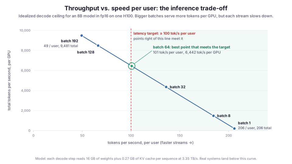
The curve is the trade-off you are always negotiating. Move left and the GPU serves more people more cheaply. Move right and each person gets a faster stream. A latency target picks the point for you: here, if every user needs at least 100 tokens per second, the best you can do is about 64 concurrent sequences and roughly 6,400 tokens per second per GPU.
Once you see inference this way, the optimizations fall into a pattern. Almost all of them do one of three things:
- Move fewer bytes per token. Quantized weights, grouped-query attention, quantized KV cache, mixture-of-experts models that only activate some of their weights per token.
- Share each byte across more tokens. Batching, and speculative decoding, which verifies several guessed tokens in one pass.
- Skip work entirely. Prefix caching reuses the prefill of a prompt the server has already seen, and routing sends easy requests to smaller models.
The inference engineer’s toolkit
These are the levers you reach for most often, what each one buys, and what it costs you.
| Lever | What it buys | What it costs |
|---|---|---|
| Continuous batching | Large throughput gains; idle batch slots refilled every step | A smarter scheduler; prefill can stall running streams |
| PagedAttention | Far less wasted KV memory, so more sequences fit | Needs runtime and kernel support (standard in modern engines) |
| Weight quantization | Fewer bytes per step, faster decode, more room for KV cache | Possible quality loss you must measure |
| KV cache quantization | More concurrent sequences per GPU | Small quality risk, mostly on long contexts |
| Prefix caching | Much lower TTFT and prefill cost for shared prefixes | Memory for cached blocks; routing must send repeat prefixes to the same replica |
| Speculative decoding | Lower TPOT, especially at small batch sizes | Extra compute; the gain shrinks as batches grow |
| FlashAttention and fused kernels | Faster attention with less memory traffic | Usually free, through the runtime |
| Chunked prefill | Steady TPOT when long prompts arrive mid-stream | Slightly higher TTFT for the long prompt |
| Tensor and pipeline parallelism | Models that don’t fit on one GPU; lower latency per token | Communication overhead; needs fast links between GPUs |
| Prefill/decode disaggregation | Each phase on hardware and settings tuned for it | Moving KV cache between machines; more parts to operate |
| Model routing | Cheap requests go to cheap models | A router that can be wrong |
A few of these deserve more than a table row.
Continuous batching is the foundation. Older servers batched whole requests and held finished slots idle until the longest request in the batch was done. Orca moved scheduling to the level of individual decode steps, so a finished request leaves and a waiting one joins on the very next step. Every serious engine does this now. If yours doesn’t, nothing else on this list matters yet.
Memory management decides concurrency. On a single GPU, the number of sequences you can run at once is the KV cache budget divided by the cache each sequence needs. PagedAttention allocates that cache in small blocks instead of reserving the maximum context length up front, and its authors report 2 to 4 times the throughput of the previous best systems at the same latency. Grouped-query attention and KV cache quantization shrink the per-sequence cost further, and every byte you save per sequence goes back into a bigger batch.
Quantization also buys concurrency. Halving the bytes per weight halves the time decode spends reading weights, and frees memory that the KV cache can use for more sequences. The cost is accuracy, and it varies by model, method and task. I don’t ship a quantized model on the strength of a perplexity number alone; I run the evals the product depends on.
Speculative decoding helps most when the GPU is underused. A small draft model guesses several tokens and the large model checks them in one pass. At low batch sizes, where the GPU has compute to spare, this can cut TPOT substantially. At high batch sizes the GPU is already busy, so the extra verification work competes with real traffic and the gain shrinks. It is a latency tool more than a throughput tool.
Parallelism is a hardware topology question. Tensor parallelism splits every layer across GPUs and talks constantly, so it belongs on GPUs joined by fast links like NVLink. Pipeline parallelism splits the model into stages and talks once per stage, so it tolerates slower links between machines. Mixture-of-experts models add expert parallelism. Picking a layout means knowing your interconnect as well as your model.
Latency, throughput and cost: picking the operating point
Every decision above lands on the same trade-off. You can’t have the lowest latency, the highest throughput and the lowest cost at the same time. In practice you fix a latency target and then maximize throughput under it, which is exactly what goodput measures.
Different products want very different points on the curve:
- Interactive chat needs a fast TTFT more than a blazing stream. A person reads at roughly 240 words a minute (Brysbaert, 2019), which is only a handful of tokens per second, so a stream much faster than that is mostly for skimming.
- Agents and tool-calling loops are different. Every token of one call’s output is input to the next step, and a task might chain dozens of calls. TPOT and TTFT compound, so agents push you to the right on the curve.
- Offline batch jobs (evaluations, document processing, synthetic data) care only about throughput and cost. Push batch sizes as high as memory allows and forget about latency.
One fleet often serves all three. Separating them, with priority classes, separate deployments, or batch work routed to off-peak capacity, is often worth more than the next kernel optimization.
How to benchmark inference without fooling yourself
Inference benchmarks are easy to run and easy to get wrong. A few rules keep the numbers honest.
Use your real length distribution. Input and output lengths decide almost everything. A benchmark with 128-token prompts tells you nothing about a RAG product that sends 6,000-token prompts. Sample lengths from production logs if you have them.
Sweep load; don’t measure a single point. Run at increasing request rates or concurrency levels and plot TTFT, TPOT and throughput against load. The knee in that curve, where latency starts climbing fast, is your real capacity.
Prefer open-loop load. A closed-loop test (N clients that each wait for a reply before sending the next request) slows itself down when the server slows down, which hides queueing. Real users don’t wait for each other. An open-loop test sends requests at a set arrival rate regardless of how the server is doing, and that shows you what happens under a traffic spike.
Report percentiles. p50, p95 and p99 for TTFT and TPOT. Averages hide the stalls users notice.
Watch for flattering caches. Sending the same prompt repeatedly turns on prefix caching and makes TTFT look excellent. Vary prompts the way real traffic does, or report cache hit rate next to the result.
Control output length. If one configuration makes the model stop earlier, it will look faster for the wrong reason. Fix the output length for speed tests, and measure quality separately.
Measure quality alongside speed. Every optimization that changes numerics (quantization, a new kernel, a runtime upgrade) can change outputs. Run a fixed evaluation set, and use an LLM-as-a-judge where exact-match scoring doesn’t fit. A speedup that costs answer quality is usually not one you can ship.
vLLM and SGLang both ship serving benchmarks that handle most of this, including request-rate sweeps and percentile reporting. Use them as a starting point and feed them your own traffic shape.
Running inference in production
A tuned engine on one GPU is a lab result. Production adds everything around it.
Autoscale on the right signal. CPU usage means almost nothing for a GPU service, and nvidia-smi utilization isn’t much better. Scale on what predicts user pain: the number of requests waiting in the queue, KV cache usage, or TTFT itself. Serving engines expose these as metrics, and tools like KEDA can scale on them.
Plan for cold starts. A new replica has to get a GPU, pull a container image, and load tens or hundreds of gigabytes of weights before it can serve. That can take minutes. Keep weights close (local NVMe or a nearby cache), keep a warm buffer of replicas, and be honest about whether scale-to-zero fits your latency targets.
Drain gracefully. An LLM response can stream for a minute. A rollout that kills pods without waiting cuts users off mid-answer. Stop sending new requests to a replica, let in-flight streams finish, then shut down. The mechanics are in graceful shutdown on Kubernetes, and a readiness probe should only pass once the model is loaded and warmed up.
Refuse work cleanly when full. When the KV cache fills up, engines start preempting running sequences and recomputing them later. A little of that is fine. A lot of it means latency spikes for everyone. Admission control that returns a fast “try again” beats accepting every request and serving all of them badly. Per-tenant rate limits keep one noisy client from filling the cache for everyone.
Route with caches in mind. Prefix caching only helps if requests that share a prefix land on the replica that holds it. Plain round-robin scatters them. Routing on a hash of the prefix, with consistent hashing so that adding a replica doesn’t reshuffle every key, keeps hit rates high as the fleet scales.
Instrument every request. Log queue time, TTFT, TPOT, input and output token counts, and cache hits per request, and trace the path through your gateway and engine. When latency jumps, you want to know within minutes whether it is longer prompts, more traffic, a lower cache hit rate, or a sick GPU.
The failures you will see most often are out-of-memory errors during the prefill of an unusually long prompt, multi-GPU jobs hanging on a collective operation when one GPU misbehaves, latency creeping up as average prompt length grows without anyone noticing, and quality changing after a runtime upgrade that nobody evaluated. Each of these is cheaper to catch with a dashboard or a CI eval than in a user complaint.
Skills you need to become an inference engineer
There is no single path into the role. People arrive from backend engineering, from HPC, from ML research and from GPU programming. The ones who do well tend to have most of the following.
- Transformer internals at the level of tensors. You should be able to sketch the shape of every tensor in a forward pass and know where these fit: attention and the KV cache, grouped-query attention, RoPE, mixture-of-experts, sampling and tokenization.
- GPU fundamentals. High-bandwidth memory versus on-chip SRAM, streaming multiprocessors, tensor cores, what a kernel launch costs, and how to read a spec sheet and predict whether a workload will be compute-bound or memory-bound.
- One serving engine, in depth. Read the scheduler and the KV cache manager of vLLM or SGLang, not just the docs. When a setting misbehaves under load, you will want to know what the code does with it.
- Profiling. The PyTorch profiler, NVIDIA Nsight Systems for the timeline, Nsight Compute for individual kernels, and DCGM metrics for fleets. Most performance work is finding out where the time really goes.
- Enough kernel programming to read and change kernels. CUDA or Triton. Not every inference engineer writes kernels every week, but you need to understand what a fused kernel saves and when a custom one is worth the maintenance.
- Distributed systems. Collective communication (NCCL), parallelism layouts, load balancing, cache-aware routing, and failure handling across machines.
- Production infrastructure. Scheduling GPUs on Kubernetes, autoscaling, rollouts and observability.
- Measurement discipline. Designing benchmarks, reading percentiles, and distrusting any single number, including your own.
If you want a project that touches all of it, try this:
- Serve a 7B or 8B open model with vLLM or SGLang on a single GPU.
- Benchmark it with an open-loop load test at several request rates and plot TTFT, TPOT and throughput.
- Predict the decode ceiling with the formula above, and explain the gap between prediction and measurement.
- Quantize the model. Measure the speedup and the quality change on a small eval set.
- Turn on prefix caching and send traffic with a shared system prompt. Watch TTFT drop.
- Add speculative decoding and find the batch size where it stops helping.
- Move to two GPUs with tensor parallelism and measure what the communication costs you.
By the end you will have run most of the experiments an inference engineer runs in their first months on the job, and you will have numbers to talk about in an interview.
Inference engineering FAQ
What is an inference engineer?
An inference engineer is a software engineer who specializes in running trained models in production. They own the latency, throughput, reliability and cost of model serving, working across GPU hardware, serving engines, batching and memory management, and the infrastructure that scales it all.
Is inference engineering the same as MLOps?
No, though they overlap. MLOps covers the lifecycle around a model: training pipelines, versioning, deployment workflows. Inference engineering goes deeper into the serving runtime itself, the part where milliseconds and GPU memory decide whether the product is fast and affordable.
Do inference engineers need to know CUDA?
It helps a lot, but not everyone writes kernels. Platform-focused inference engineers spend more time on scheduling, routing, autoscaling and benchmarking. Runtime-focused ones read and write CUDA or Triton regularly. Everyone in the role needs to understand what the GPU is doing well enough to predict performance.
What tools do inference engineers use?
Serving engines such as vLLM, SGLang, TensorRT-LLM and llama.cpp; profilers such as Nsight Systems, Nsight Compute and the PyTorch profiler; load-testing and benchmarking tools; Kubernetes and an autoscaler; and a metrics and tracing stack for per-request latency.
Why is LLM inference so expensive?
Because decode is limited by memory bandwidth, not compute. Each generated token requires reading the model’s weights and the request’s KV cache from GPU memory. Unless many requests share those reads through batching, an expensive GPU spends most of its time waiting. Most of inference engineering is about making that sharing as efficient as possible.
Is inference engineering only about LLMs?
No. The same work applies to speech recognition, image generation, vision models, embeddings and recommendation systems. LLMs made the role prominent because their memory footprint, autoregressive decoding and long, variable-length requests make naive serving unusually expensive.
Where I start with a new deployment
When someone hands me a new model to serve, I don’t start in a config file. I write down four numbers: the size of the weights, the KV cache per token, the memory bandwidth of the card, and the latency target. From those I sketch the curve above on paper and mark where the target cuts it. That gives me a ceiling for throughput per GPU before I’ve loaded anything.
Then I measure, with traffic that looks like the real thing, and most of the work after that is explaining why reality landed below the line: a long-prompt burst that stalls decode, a cache hit rate lower than expected, a kernel that isn’t the one I thought was running. Batching, quantization, KV cache management, speculative decoding, prefix caching and parallelism are all ways to move fewer bytes, share them across more tokens, or skip the work. Knowing which one to reach for, and proving it helped, is inference engineering.
Diagrams by M. Hassan Ahmed, released under CC0. No external image was used for this post; the figures are original work by the author.