How Byte-Pair Encoding Tokenizes Text for LLMs
Byte-pair encoding turns text into the tokens an LLM bills and reasons over. How BPE merges are learned, why token counts drive cost, and where it breaks.

You count characters; the model counts tokens. That gap sits behind a surprising number of the bugs and bills that appear once an LLM is in production:
- a prompt that fit yesterday now overflows the context window,
- a request costs twice what a similar one did,
- the model insists “strawberry” has two r’s.
None of these mean the model is dumb. The model works on a representation of your text that you never see, and a tokenizer produces that representation. For almost every current model, the tokenizer is some variant of byte-pair encoding (BPE).
This post is for engineers who send text to an LLM and want to know what happens to it before the first layer of the network sees it. I build the algorithm from a tiny worked example you can run, show how the same mechanism explains the cost and context math you already deal with, and then spend time on the failure modes, because that is where tokenization stops being trivia and starts costing you.
I hit this constantly on the retrieval side of Archi, the RAG copilot I worked on for CMS computing operations at CERN. There, one token budget has to cover logs, code, and ticket text in more than one language.
A token is neither a word nor a character
The first instinct is that a token is a word. It isn’t. Splitting on whitespace gives you a vocabulary that never ends, because every typo, every run_id, and every hostname is a new word. It also gives you no way to represent a word you have not seen before.
The opposite instinct, one token per character, gives you a tiny fixed vocabulary. But sequences become enormous, and you throw away the fact that pieces like “ing” and “tion” are worth learning as units.
BPE sits in between. A token is a subword: a chunk of characters that appeared often enough in the training text to earn its own slot in the vocabulary.
- Common words end up as one token.
- Rare words get split into a few pieces.
- Genuinely novel strings fall back to smaller and smaller pieces, down to single bytes if necessary.
That last property is what makes BPE usable in practice. The tokenizer can encode literally any input and never fails on an out-of-vocabulary word.
Where BPE came from
The algorithm is older than its deep-learning use. Philip Gage described byte-pair encoding as a data-compression scheme in 1994: repeatedly replace the most frequent pair of adjacent bytes with a new byte, and the stream gets smaller (overview on Wikipedia).
In 2016, Sennrich, Haddow and Birch borrowed that idea for neural machine translation. They used the same greedy merge procedure to build a subword vocabulary instead of a compression table (Sennrich et al., “Neural Machine Translation of Rare Words with Subword Units,” ACL 2016). That paper is the reason nearly every model you use today tokenizes the way it does.
GPT-2 added one refinement that matters: it runs BPE over raw bytes instead of Unicode characters (Radford et al., 2019). The base vocabulary is the 256 possible byte values. As a result, there is no character the tokenizer cannot represent, no <unk> (unknown) token, and no special handling for emoji or for scripts the training set barely covered. OpenAI’s tiktoken and most open models use this byte-level flavor.
How the merges are learned
Training a BPE tokenizer is just counting:
- Take a corpus and split every word into characters, plus an end-of-word marker.
- Find the most frequent pair of adjacent symbols across the whole corpus.
- Merge that pair into a single new symbol and record the merge.
- Repeat the find-and-merge step a fixed number of times.
The ordered list of merges is your tokenizer.
Here is the whole thing on a four-word toy corpus, small enough to check by hand. The word frequencies are made up; the merges are not. The code runs five rounds of merging and prints each merge along with how often that pair occurred.
import collections

corpus = {"low": 5, "lower": 2, "newest": 6, "widest": 3}

# each word starts as characters + an end-of-word mark
vocab = {" ".join(w) + " ·": f for w, f in corpus.items()}

def most_frequent_pair(vocab):
    pairs = collections.Counter()
    for word, freq in vocab.items():
        syms = word.split()
        for a, b in zip(syms, syms[1:]):
            pairs[(a, b)] += freq
    return pairs.most_common(1)[0]

merges = []
for _ in range(5):
    (a, b), count = most_frequent_pair(vocab)
    merges.append((a, b))
    bigram, joined = f"{a} {b}", a + b
    vocab = {w.replace(bigram, joined): f for w, f in vocab.items()}
    print(f"{a} + {b}  (freq {count})  ->  {joined}")
Run it, and the counts force this order:
e + s   (freq 9)  ->  es
es + t  (freq 9)  ->  est
est + · (freq 9)  ->  est·
l + o   (freq 7)  ->  lo
lo + w  (freq 7)  ->  low
e s wins first because it appears in both newest (×6) and widest (×3), nine times in total, more than any other pair. Once es exists, es t becomes the most frequent pair, and so on.
The tokenizer never decided that “est” is a meaningful English suffix. It fell out of the arithmetic. That is the whole trick: linguistically sensible pieces emerge from frequency alone, with no grammar and no word list.
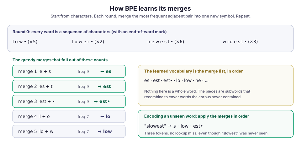
The payoff is generalization. To encode a word the corpus never contained, you apply the learned merges to it in the order they were learned. The encode function below does exactly that, one merge rule at a time:
def encode(word, merges):
    syms = list(word) + ["·"]
    for a, b in merges:
        i, out = 0, []
        while i < len(syms):
            if i < len(syms) - 1 and syms[i] == a and syms[i + 1] == b:
                out.append(a + b); i += 2
            else:
                out.append(syms[i]); i += 1
        syms = out
    return syms

encode("slowest", merges)   # -> ['s', 'low', 'est·']
slowest was not in the training corpus, yet it encodes cleanly into three known pieces. This is the property that lets a fixed vocabulary of ~100K to 200K tokens cover the effectively infinite space of strings people actually type.
Why token counts drive cost, context, and memory
Everything downstream of the tokenizer is measured in tokens, not characters. The split you cannot see is the split you pay for, and it shows up in three places.
Cost. API pricing is per token in and per token out. A rough rule for English is about four characters per token, but it is only a rule of thumb. The honest way to budget is to run the real tokenizer over representative inputs, not to divide len(text) by four. Code, JSON, and long identifiers tokenize much less efficiently than prose, because they are full of rare substrings and runs of whitespace.
Context window. The window’s size is a token count. When a RAG answer stuffs retrieved chunks into the prompt, tokenization decides what fits, so measuring your chunks in characters and hoping is how you get truncated context. This is one more reason I care about retrieval quality: tighter retrieval spends fewer tokens to say the same thing.
GPU memory. On self-hosted models, the KV cache (the stored attention keys and values for every token so far) grows linearly with the number of tokens in the sequence, not the number of characters. A tokenizer that splits your text into more pieces fills VRAM faster.
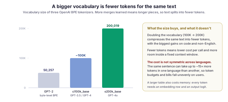
The vocabulary size a model was trained with sets the exchange rate between text and tokens. A larger vocabulary learns more merges, and longer ones, so the same text collapses into fewer tokens. OpenAI’s tokenizers show the trend directly:
- GPT-2 shipped with 50,257 tokens.
cl100k_base(GPT-3.5 and GPT-4) roughly doubled that to about 100K.o200k_base(GPT-4o) doubled it again to 200,019, with the biggest compression gains on code and non-English text.
Failure modes worth knowing
This is where tokenization earns its place in a debugging session.
Character-level tasks. The model reasons over tokens, not letters. A word like “strawberry” may become a handful of subword pieces (something along the lines of str + aw + berry), and the model never sees the three separate r’s inside them. That is why LLMs are worst at exactly the tasks that depend on letters: counting them, reversing a string, or catching a specific character. It is not a reasoning gap; the tokenizer threw the information away. If you need character-level correctness, do it in code, not in the prompt.
The multilingual tax. The merges are learned mostly from English-heavy text, so English compresses well and other languages do not. Petrov et al. measured the same sentence taking up to about 15× more tokens in some languages than in others (Petrov et al., “Language Model Tokenizers Introduce Unfairness Between Languages,” NeurIPS 2023). That is not cosmetic. It means slower responses, less content in the window, and a higher bill for the same request, and it all falls on the languages that were already underrepresented. If your users write in more than one language, your token budget is not evenly funded.
Numbers tokenize badly. Digits get split into pieces that have nothing to do with place value, which is part of why arithmetic on long numbers is shaky. Some newer tokenizers deliberately split numbers into single digits or fixed-size groups to make this less erratic, but you cannot assume it.
Leading spaces are part of the token. In byte-level BPE a leading space is usually attached to the following word, so "hello" and " hello" are different tokens. Trailing whitespace in a prompt can nudge the model into a worse continuation than you expect. When output looks subtly off, check whether you appended a stray space.
Glitch tokens. Some tokens exist in the vocabulary but the model almost never saw them during training, because the tokenizer and the model were trained on different data. Hitting one of these under-trained tokens can produce bizarre, off-topic output; the most famous is SolidGoldMagikarp. There is a whole method for hunting them down (Land & Bartolo, “Fishing for Magikarp,” 2024). You will rarely trigger one by accident, but if a specific rare string makes a model behave strangely, suspect a glitch token.
Tradeoffs, and what I keep in mind
A bigger vocabulary shortens sequences, but it is not free. Every token needs a row in the embedding table and a slot in the output layer, so doubling the vocabulary grows both. Past a point, you are spending parameters to shave tokens off text nobody sends.
There is also a slower-moving cost. The tokenizer is effectively frozen once a model is trained on it, so a vocabulary tuned for 2019’s web ages as usage shifts. Some newer models are moving toward learned or unigram-based tokenizers to soften a few of BPE’s rough edges (the Hugging Face tokenizer summary lays out the alternatives). Still, BPE is what you will meet most often.
The practical habits are short:
- Measure prompt length with the model’s actual tokenizer, never with a character count.
- If you serve multiple languages, budget for the worst-case language, not the average.
- Keep character-level logic in code, where characters still exist.
- To make the mechanism stick, work through Andrej Karpathy’s minbpe, which builds a real one from scratch. It is worth an afternoon.
None of this is exotic. BPE is a greedy frequency count that discovers useful subwords on its own. Once you can see the pieces your text turns into, the token bill, the context overflow, and the model that cannot count r’s all read as the same fact from different angles. I ran this arithmetic often, across the CMS workflow tooling and on the long-context side of Archi, where knowing what a token actually is decided how many logs and docs I could afford to send.
Diagrams by M. Hassan Ahmed, released under CC0. No external image was used in this post.