Prefill vs Decode: Two Phases of LLM Inference

The first time I sat with the latency numbers behind Archi, the retrieval copilot I worked on for CMS computing operations at CERN, one pattern stood out. A short question with a long retrieved context waited a beat before anything appeared, then streamed its answer smoothly. A short question with almost no context started faster, but streamed at the same steady pace. The time before the first word and the time between words are set by two different things, and they don’t move together.

That gap has a name. An LLM answers a request in two phases with completely different performance characteristics: prefill, which reads the prompt, and decode, which writes the answer. Prefill is limited by how much math the GPU can do. Decode is limited by how fast the GPU can read memory.

This post is for engineers who already call an LLM, whether they serve models themselves or go through an API, and now need to reason about its latency. The split also explains why a longer prompt taxes your latency budget more than a longer answer does. I’ll walk through what each phase does, why they hit different hardware limits, how that shows up in the metrics you actually measure, and what you can do about it.

The two phases at a glance

An autoregressive language model generates text one token at a time, and each new token depends on every token before it. That single fact forces the two-phase shape.

When your prompt arrives, the model has to process all of it before it can produce anything. It runs one forward pass over the entire prompt at once. That pass computes the attention keys and values for every token and stores them in the KV cache. This is prefill, and it ends by producing exactly one token: the first token of the answer.

From there the model is in decode. It takes the token it just generated, runs a forward pass for that single position, produces the next token, appends it, and repeats. Every step reuses the keys and values already in the KV cache, so it never re-reads the prompt. One pass, one token, in a loop, until the model emits a stop token or hits the length limit.

The timeline below shows one request. TTFT and TPOT are the two latency metrics covered later in the post: time to first token and time per output token.

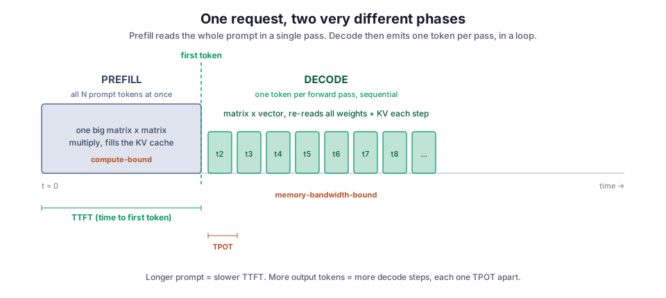
The shapes on that timeline are the whole story. Prefill is one wide block whose width grows with the prompt. Decode is a train of identical small steps, one per output token. A longer prompt makes the block wider; a longer answer makes the train longer.

Prefill: the whole prompt in one pass

Prefill handles every prompt token in the same pass, so its core operation is a matrix times another matrix: the model’s weights against a stack of hundreds or thousands of token vectors. Modern GPUs are extremely good at exactly this. The weights are read from high-bandwidth memory (HBM) once, and that one read is shared across all the tokens in the batch, so the arithmetic units stay busy doing useful work.

That is what “compute-bound” means: the limiting resource is FLOPs, the raw math throughput, not memory traffic. The roofline model is the standard way to picture this. An operation with high enough arithmetic intensity (math per byte loaded) sits under the compute ceiling, so the ALUs (arithmetic logic units, the parts of the chip that do the math) are what limit it. Prefill is that kind of operation.

The consequence for latency is direct. Prefill cost scales with prompt length, so a long prompt means a longer wait before the first token appears. That’s why stuffing more retrieved chunks into a RAG prompt isn’t free, even when the model’s context window has room: every extra token of context is more prefill work, paid before the user sees anything. In Archi this is a real tradeoff. The honest answer often needs several retrieved documents, and each one pushes the first token further out.

Decode: one token at a time

Decode runs the same forward pass, but the math is lopsided. Each step processes a single new token, so the operation is a matrix (the weights) times a vector (one token’s worth of activations). The model still has to read every weight from HBM to compute that one token. Read the entire model, do one token of work, give the ALUs almost no math to chew on, repeat.

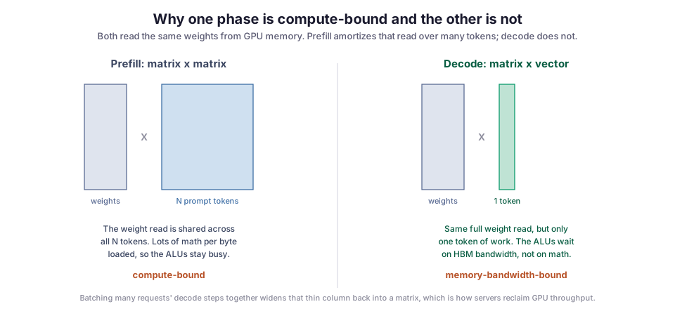
Now the bottleneck is memory bandwidth, not compute. The GPU spends most of each decode step waiting to pull weights and the growing KV cache out of HBM, while its expensive compute units sit mostly idle. Databricks states this split plainly in their inference performance guide: “Generating the first token is typically compute-bound, while subsequent decoding is a memory-bound operation.” Because decode is memory-bound, the time per token tracks how fast you can move bytes. That is why memory bandwidth utilization is the metric people optimize decode against.

This is also why single-request decode wastes a data-center GPU. You bought a card that can do enormous matrix math, and decode hands it a matrix-times-vector. The fix is batching, which I’ll come back to.

How the phases show up in your metrics

The two phases map cleanly onto the two latency numbers worth tracking. Keeping them separate is the single most useful habit when you debug LLM latency (a good reference on the metrics):

• TTFT (time to first token) is essentially the cost of prefill. Prompt length dominates it, along with how loaded the server is when your request lands.
• TPOT (time per output token), sometimes called inter-token latency, is the cost of one decode step. It sets how fast the answer streams once it starts.

Total time for a response is roughly TTFT + (output_tokens - 1) * TPOT. Two knobs, two phases. A slow start is a prefill problem, a slow stream is a decode problem, and they call for different fixes.

If you consume a streaming endpoint, you can measure both from the client. The script below times the same server-sent events stream I use to push tokens to the Archi frontend, from the caller’s side. It records the arrival of the first non-empty chunk as TTFT, then averages the gaps between consecutive chunks as TPOT:

import time
from openai import OpenAI

client = OpenAI()

start = time.perf_counter()
ttft = None
token_times = []

stream = client.chat.completions.create(
    model="gpt-4o-mini",
    messages=[{"role": "user", "content": prompt}],
    stream=True,
)

for chunk in stream:
    delta = chunk.choices[0].delta.content
    if not delta:
        continue
    now = time.perf_counter()
    if ttft is None:
        ttft = now - start          # prefill latency, roughly
    token_times.append(now)

# average gap between streamed tokens = TPOT, roughly
gaps = [b - a for a, b in zip(token_times, token_times[1:])]
tpot = sum(gaps) / len(gaps) if gaps else 0.0
print(f"TTFT: {ttft*1000:.0f} ms   TPOT: {tpot*1000:.1f} ms/token")

Run that across prompts of different lengths and the shape falls right out: TTFT climbs with prompt size while TPOT stays roughly flat. So if TPOT is what’s hurting, a shorter prompt won’t save you. That’s a decode-side problem.

What you can do about it

Once you know which phase is slow, the options narrow down to three.

Skip repeated prefill with prefix caching

Often the front of your prompt is stable: a long system prompt, few-shot examples, a fixed instruction block. Then you can stop paying to recompute it. Prefix caching lets the server reuse the KV cache for that shared prefix instead of running prefill on it every call, so it’s prefill you skip.

For RAG this is also an argument about prompt layout. Keep the fixed scaffolding at the top and the volatile retrieved chunks lower down, so the cacheable part stays contiguous.

Batch decode steps together

Decode is the phase batching exists to rescue. A single request underuses the GPU, so servers run many requests’ decode steps together, and the thin one-token column widens back into a matrix.

Continuous batching admits and retires requests at the granularity of individual decode steps, instead of waiting for a whole batch to finish. It is standard in serving stacks like vLLM, and per the same Databricks writeup it buys an order of magnitude more throughput than naive batching. You don’t control this on a hosted API, but it explains why your TPOT gets worse when the provider is busy: you’re sharing decode batches with everyone else.

Put the phases on separate GPUs

The last option is to stop making the two phases share a GPU at all. They interfere, because one is compute-hungry and the other bandwidth-hungry. DistServe (OSDI ‘24) puts them on separate pools of GPUs that scale and tune independently, and reports large gains in requests served under fixed latency targets. That’s an infrastructure decision rather than something you reach for in an app, but it’s the clearest proof that these are two different workloads wearing one API.

What bites you

A few failure modes follow directly from the split, and I’ve hit most of them.

Blaming the wrong phase. This is the most common. A slow experience gets reported as “the model is slow,” but slow-to-start and slow-to-stream have nothing in common. Measure TTFT and TPOT separately before you change anything, or you’ll shorten prompts to fix a decode problem and wonder why nothing improved.

Prompt bloat. This one creeps up on you. Every retrieved chunk, extra few-shot example, and verbose system prompt is prefill you pay on every single call. The context window allows it, so context keeps getting added, and first-token latency drifts up with no single obvious cause. The KV cache grows with that same prompt length, so you’re spending both latency and memory.

Expecting a bigger GPU to speed up streaming. This is the one that costs money. If decode is memory-bandwidth-bound, a card with more FLOPs but similar bandwidth barely moves TPOT. Compare memory bandwidth on the spec sheet, not peak TFLOPs; it’s easy to buy the wrong axis.

Closing: profile the two phases separately

The prefill/decode distinction quietly explains a dozen other things:

• why prompt length hurts more than answer length at the start,
• why prompt caching pays off,
• why a batched server has better throughput but not better single-request latency,
• why the KV cache exists at all.

For Archi, keeping TTFT and TPOT as separate numbers is what lets me reason about whether an extra retrieved document is worth the wait it adds, and answer that honestly rather than by feel.

If you’re building on top of LLMs, whether that’s a RAG copilot or the CMS workflow tooling I maintained at CERN, the same rule holds: profile the two phases separately, and fix the one that’s actually slow.

Further reading: DistServe (OSDI ‘24) on disaggregating the two phases, and Databricks’ LLM inference performance guide on the metrics. Diagrams are my own; no external image was used.