How Roaring Bitmaps Make Filters Fast

Every filter you type into a search box turns into a set of integers somewhere. Ask OpenSearch for documents where site = FNAL and status = failed, and each clause resolves to a set of internal document IDs. The engine intersects those sets, and whatever survives is what you get back. The hard part is not the matching. It is storing those ID sets in a form that intersects fast and does not blow up memory when a filter matches ten million rows.

I ran into this from the retrieval side. On Archi, the RAG copilot I worked on for CMS computing operations at CERN, almost every question is scoped: one subsystem, one logbook, the last week of tickets. When I wrote up metadata filtering for vector search, I kept describing the filter as “a set of allowed IDs” and moving on. This post is about the data structure behind that set. The choice is not obvious, and the wrong one shows up as either slow queries or a memory graph that climbs all day.

The post is for engineers who work with a search or analytics engine and have wondered why Lucene, ClickHouse, and Druid all reached for the same structure: the roaring bitmap. It covers how roaring stores a set, why its operations are fast, where you are already using it, and when it is the wrong tool.

Why neither arrays nor plain bitmaps work

Start with the two obvious ways to store a set of document IDs. Both fail, at opposite ends.

A sorted array of integers. A filter matching 40 rows costs 160 bytes, and it intersects with another set by walking both lists in order (a merge). Clean and small. Now suppose the filter matches 8 million rows out of 10 million. The same array is 32 MB for one clause, held in RAM for each cached filter. Intersecting two dense arrays means walking both end to end.

A bitmap. Store one bit per possible document, set to 1 if the document matches. Intersection becomes a bitwise AND across machine words, which is about as fast as computers get. But the size no longer depends on how many rows match. A bitmap over 10 million documents is 1.25 MB whether the filter matches everything or one row. Cache a few thousand sparse filters and you pay megabytes each for sets that hold three IDs.

Arrays win when a set is sparse; bitmaps win when it is dense. A real search index has both kinds of filter in flight at the same time. What you want is a structure that automatically uses the right representation in each region of the ID space, without you having to choose.

The roaring idea: split into chunks, then pick a container per chunk

Roaring bitmaps come from a 2016 paper by Daniel Lemire and colleagues, Better bitmap performance with Roaring bitmaps, later extended in Roaring Bitmaps: Implementation of an Optimized Software Library. The core idea is small, and it is the whole trick.

Take a 32-bit integer and cut it in half:

• The high 16 bits pick a chunk.
• The low 16 bits are the value inside that chunk.

Each chunk therefore covers a fixed window of 65,536 possible values (2^16). The bitmap keeps a sorted list of only the chunks that actually contain something. For each chunk, it decides independently how to store that chunk’s values, picking whichever of three container types is smallest for the density it sees.

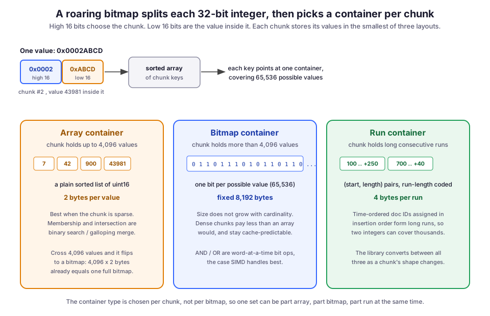
The three containers, and when each one is used:

• Array container. A plain sorted array of 16-bit values, 2 bytes each, used while a chunk is sparse. Membership is a binary search; intersection with another array is a merge.
• Bitmap container. A fixed 8,192-byte bitmap (65,536 bits, one per possible value in the chunk), used once a chunk gets dense. Its size never changes with how many values it holds.
• Run container. A list of (start, length) pairs at 4 bytes per run, which is run-length encoding of the values. It is used when a chunk is mostly long consecutive spans, where two integers can stand in for thousands of IDs.

Where the array/bitmap switch happens

The crossover between array and bitmap is not a guess; it is arithmetic. An array container caps at 4,096 values. At exactly 4,096 values it costs 4,096 × 2 = 8,192 bytes, which is precisely the size of one bitmap container. Below that, the array is smaller. Above it, the bitmap is smaller and stops growing.

So the moment a chunk’s cardinality (its count of values) crosses 4,096, the library converts the array into a bitmap. It converts back if the chunk thins out again. The library picks a run container by a similar size comparison, when the values form few enough runs to beat both.

The key consequence: the container type is chosen per chunk, not per set. A single roaring bitmap over your corpus can be all three at once:

• an array container where doc IDs are sparse,
• a bitmap container where they are dense,
• a run container over a block of sequential IDs.

The structure adapts to the shape of your data in each 65,536-wide window instead of committing to one representation for everything.

Why the containers make operations fast

Compression you have to undo before you can use the data is a tax. Roaring avoids it: operations run directly on the compressed form, and each operation picks its algorithm from the pair of container types involved.

• Bitmap and bitmap intersect with a word-at-a-time bitwise AND, exactly the pattern SIMD (single instruction, multiple data) units are built for.
• Array and array merge like two sorted lists.
• Array and bitmap intersect by looking up each array element’s bit in the bitmap. That is cheap, because the array is the small side.

The library carries a specialized routine for each combination. An AND across a whole bitmap is really a sequence of per-chunk operations, each one already the right algorithm for its case. On intersection, chunks that exist in only one of the two bitmaps are skipped entirely, because a missing chunk contributes nothing.

That is why site = FNAL AND status = failed stays quick even when one side is a huge dense set and the other is a scattering. Each side is stored in whatever container fits it, and the intersection routine handles each pair of containers in its own best way.

Where you have already been using this

If you run OpenSearch or Elasticsearch, you have been relying on roaring bitmaps without knowing it. Both are built on Apache Lucene, and Lucene’s query cache stores filter results as roaring-style doc-ID sets.

Look at Lucene’s LRUQueryCache. When it caches the documents matching a filter, it keeps them in a RoaringDocIdSet for sets below roughly 1% density and switches to a fixed bitset above that. That is the same chunk-and-pick idea, tuned for cached filters. It is why a repeated filter clause in an OpenSearch query gets cheaper after the first run, and why the cache does not fall over when one of those filters matches most of the index.

The list of systems that made this choice is long, and that is not a coincidence. Lucene, ClickHouse, Apache Druid, Apache Pinot, InfluxDB, and Spark have all used roaring bitmaps for set-valued indexes and query execution. When you filter a dashboard in any of them, an intersection of roaring bitmaps is usually what runs.

For me, the connection is the pre-filter step in filtered vector search. Before an approximate-nearest-neighbor walk, you often want the set of documents that pass the metadata filter, so the graph search only visits allowed candidates. That allow-set is exactly the kind of integer set roaring holds well. Building it from cached per-attribute bitmaps is an intersection, not a scan. The same structure that speeds up a keyword filter also feeds the vector side.

Trying it in Python

The reference C library is CRoaring, and pyroaring wraps it. The short session below builds one dense and one sparse set, prints their memory footprint, and intersects them.

from pyroaring import BitMap

# A dense filter: "documents 0 through 5 million matched"
dense = BitMap(range(0, 5_000_000))

# A sparse filter: a few thousand scattered IDs
import random
sparse = BitMap(random.sample(range(0, 10_000_000), 3_000))

print(dense.get_statistics()["n_bytes"])   # tens of KB, not megabytes
print(sparse.get_statistics()["n_bytes"])  # a few KB

# The operation a filter query is really doing
hits = dense & sparse          # intersection, container by container
print(len(hits))

Two things to notice:

• Size. The dense set of five million contiguous IDs takes tens of kilobytes. A raw bitmap would need 625 KB, and an integer array would need 20 MB. The difference is that those contiguous IDs collapse into run containers.
• The intersection. It is not a loop over IDs; it is a single &. Underneath, it dispatches per chunk to bitmap-AND, array-merge, or run logic as appropriate.

get_statistics() also tells you how many of each container type your set decomposed into. That is the honest way to reason about a production bitmap. If a set you expected to be tiny is full of bitmap containers, your IDs are denser or more scattered than you thought.

Tradeoffs and failure modes

Roaring has sharp edges. Here are the ones I would keep in mind before reaching for it.

It needs reasonably clustered integer IDs. Roaring stores sets of integers, and everything above depends on those identifiers clustering. Doc IDs handed out in insertion order cluster beautifully and run-encode almost for free. Cryptographic hashes spread uniformly across the full 2^32 space do not. Every chunk holds a handful of values, you get thousands of half-empty array containers, and you pay roaring’s bookkeeping overhead for very little compression. If your keys are random 64-bit hashes, map them to dense internal IDs first, which is what Lucene does with its per-segment doc IDs.

It is overkill for small sets. For very small sets, a plain set or sorted array is simpler and just as fast. Roaring earns its keep at scale and when you intersect and union constantly, not for a filter that matches twelve rows once.

It answers exact membership, nothing more. If your real question is “have I probably seen this ID?” under a memory budget, you want a Bloom filter. If it is “roughly how many distinct IDs are there?”, you want HyperLogLog. Using roaring there means paying to store exact members you were willing to approximate.

Serialized bitmaps are not portable by default. If you serialize bitmaps and read them from another language, use the portable format spec rather than a library’s native dump. Otherwise a Java writer and a Python reader will disagree.

What I would keep in mind

The lesson that carried over to how I think about the rest of my stack: the win did not come from a cleverer compression algorithm. It came from refusing to pick one representation for the whole set. Roaring chooses per region, from the local density, with cheap conversions when that density changes. A sparse corner stays a list, a dense corner becomes a bitmap, a sequential corner becomes a run, and each operation meets every region in its best form.

On Archi, a filter can select 0.1% of the corpus for one subsystem and 40% for another. There, that per-region instinct is the difference between a filter cache that helps and one that quietly eats memory. If you are building filtering on top of OpenSearch or any Lucene-based engine, know that this structure is already carrying your filters, and check get_statistics() when a set behaves in a way you did not expect.

The diagram in this post was generated for it. No external image was used.