Metadata Filtering in RAG Vector Search

Most RAG bugs I have chased were not embedding-quality problems. They were filter problems. Someone asks the copilot about a transfer error at a specific site, and the answer quotes a fix from a different site two years earlier. Everyone concludes the retrieval is bad. It usually is not: the nearest vectors were fine. The system just failed to restrict the search to the rows that were actually relevant.

This post is for engineers building retrieval on a vector store who need results scoped by structured attributes: a site, a date range, a document type, an access level. It covers:

• the three ways an engine can combine a metadata filter with an approximate-nearest-neighbor (ANN) search, and why the naive one quietly hurts recall;
• why filtering an HNSW graph is harder than it looks;
• how the choice plays out in Postgres, Qdrant, and OpenSearch.

The running example is Archi, the retrieval copilot I worked on for CMS computing operations at CERN. There, “only entries from this site, this year” is part of almost every query.

Why vector distance alone is not enough

A vector index answers one question well: given this query vector, which stored vectors are closest? It knows nothing about where a chunk came from, such as a 2021 logbook for a different site. So once your data has structure (and operations data always does), you need to satisfy two constraints at once: close in embedding space and matches these attributes.

The three strategies below differ only in when the engine applies the filter relative to the search. That ordering decides whether you get correct results, fast results, or neither.

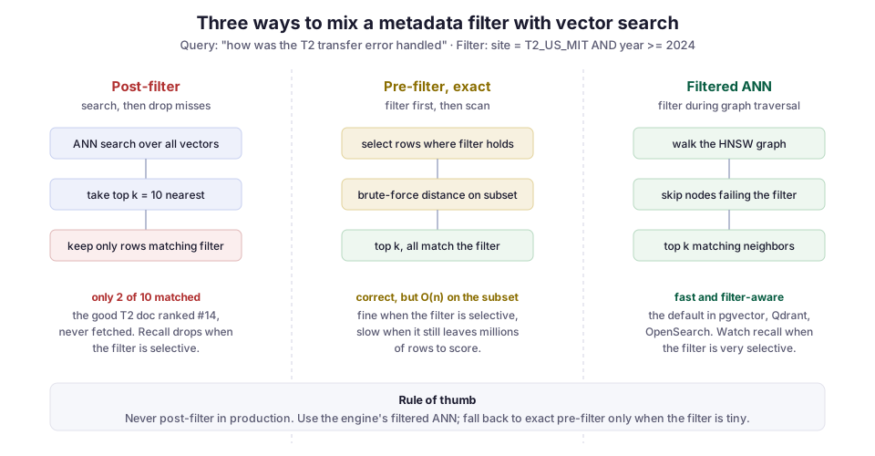
Strategy 1: post-filter, and why it fails quietly

The tempting version, especially when you bolt a filter onto an existing search, is to run the vector query, take the top k, then throw away the rows that do not match. This is a post-filter, sometimes called filter-after-search. The query below is the kind that looks correct but behaves this way:

-- pgvector: search first, filter the result set. Looks fine, isn't.
SELECT id, body
FROM chunks
WHERE embedding <=> :query_vec < 1.0        -- distance, computed on ALL rows
  AND site = 'T2_US_MIT' AND year >= 2024   -- filter applied to top-k output
ORDER BY embedding <=> :query_vec
LIMIT 10;

The failure mode is not an error. It is silent recall loss (recall being the share of truly relevant documents that come back). Here is how it happens:

1. Say site = 'T2_US_MIT' covers 3% of your corpus, and the query is generic enough that most of the closest vectors come from busier sites.
2. The ANN search returns its ten nearest neighbors, and eight of them come from other sites.
3. The filter removes those eight, leaving two rows.
4. The genuinely relevant MIT document sat at rank fourteen. It was never fetched, so it never had a chance.

You asked for LIMIT 10 and got two. Nobody sees a stack trace; you just see a worse answer.

You can paper over this by over-fetching: request k = 200, filter down, and hope enough rows survive. But that is a guess, and the more selective the filter, the worse the guess gets. For a filter matching 0.1% of rows, you might fetch thousands and still come up short. Post-filtering is fine for a demo and a liability in production. Of the three options in the diagram, it is the one I would tell you never to ship.

Strategy 2: exact pre-filter

The opposite order is to filter first, then run an exact (brute-force) distance scan over whatever survives:

-- Filter first, then score exactly on the subset.
SELECT id, body
FROM chunks
WHERE site = 'T2_US_MIT' AND year >= 2024
ORDER BY embedding <=> :query_vec
LIMIT 10;

This is always correct. Every returned row matches the filter, and because the engine scores the whole subset exactly, you get the true nearest neighbors within it.

The catch is cost. A brute-force scan is O(n) in the size of the filtered subset. If site = 'T2_US_MIT' AND year >= 2024 leaves a few thousand rows, scanning them is nothing, often faster than touching the ANN index at all. If your filter is loose and leaves several million rows, you compute millions of distances per query while the ANN index you built sits unused.

So exact pre-filter is the right tool precisely when the filter is selective. Postgres knows this: with pgvector, if the planner estimates that the filtered set is small, it skips the vector index and does exactly this scan. The trouble starts in the middle ground, with filters that are neither tiny nor loose. That is where the third strategy earns its place.

Strategy 3: filtered ANN, the one you actually want

The strategy that scales pushes the filter into the ANN search itself, so the graph traversal only ever considers nodes that satisfy the predicate. The engine wastes no distance computations on rows it will discard, and it never brute-forces a huge subset.

Why filtering an HNSW graph is hard

This sounds obvious, and it is genuinely hard to implement well. HNSW is a navigable small-world graph: search works by greedily hopping to closer and closer neighbors. When you forbid most nodes, you tear holes in that graph.

The path from the entry point to the best matching node may run through nodes that fail the filter. If the search cannot step on them, it cannot reach the destination. Recall collapses even though the matching node is in the index.

The engines that do this well spend their effort on exactly this problem: staying connected while honoring the filter. Qdrant’s team wrote a good explanation of why filtered HNSW is not just “skip the bad nodes” and how they keep the graph traversable (filtrable HNSW). Research systems like ACORN attack the same problem by searching an expanded neighborhood, so the traversal can route around filtered-out nodes.

How each engine exposes it

The practical point: you do not implement this yourself. You use an engine that treats the filter as a first-class part of the query, and you verify its recall on your own data.

pgvector (0.8+). Give the planner the filter alongside ORDER BY embedding <=> :query_vec. Iterative index scans then keep pulling from the HNSW index until enough rows pass the filter, instead of stopping at the first k (pgvector filtering docs). The query is the same as in Strategy 2; the SET line is what changes the behavior:

-- pgvector 0.8+: iterative scan keeps reading the index until the
-- filter is satisfied, rather than post-filtering a fixed k.
SET hnsw.iterative_scan = 'relaxed_order';
SELECT id, body
FROM chunks
WHERE site = 'T2_US_MIT' AND year >= 2024
ORDER BY embedding <=> :query_vec
LIMIT 10;

OpenSearch. The k-NN query takes a filter clause and applies it during the search rather than after. The engine decides between exact and approximate search based on how restrictive the filter is (efficient k-NN filtering). Archi’s retrieval runs on OpenSearch, which is why I keep coming back to it in these posts. The same index backs both the BM25 half of hybrid search and the metadata filters here. In the request below, notice that the filter sits inside the knn clause, not beside it:

{
  "size": 10,
  "query": {
    "knn": {
      "embedding": {
        "vector": [0.11, -0.04, "..."],
        "k": 10,
        "filter": {
          "bool": {
            "must": [
              { "term": { "site": "T2_US_MIT" } },
              { "range": { "year": { "gte": 2024 } } }
            ]
          }
        }
      }
    }
  }
}

Qdrant. The filter is a top-level part of the request. Usefully, Qdrant lets you build a payload index on the fields you filter by, so the predicate is cheap to evaluate during traversal (Qdrant filtering). The same site-and-year filter looks like this in the Python client:

from qdrant_client import QdrantClient, models

client.query_points(
    collection_name="chunks",
    query=query_vec,
    query_filter=models.Filter(must=[
        models.FieldCondition(key="site", match=models.MatchValue(value="T2_US_MIT")),
        models.FieldCondition(key="year", range=models.Range(gte=2024)),
    ]),
    limit=10,
)

Failure modes to know before they bite

Selective filters quietly lower recall. Filtered ANN does not escape the connectivity problem. The more of the graph your filter removes, the more likely the traversal misses the true nearest matching node. When a filter gets extreme, matching well under 1% of rows, most engines fall back to exact search for that query, which is correct but slower. Know where your engine draws that line, because query latency will jump there.

High-cardinality filters need their own index. Filtering on a field the engine must check candidate by candidate is slow. Build the field index so the predicate becomes a lookup, not a scan: a Qdrant payload index, an OpenSearch mapping with the field indexed, or a Postgres B-tree on site/year.

Range filters on timestamps are the common trap. year >= 2024 is cheap. created_at BETWEEN two arbitrary instants across a huge table is not, unless the field is indexed and the engine can use it during traversal. In Archi, we filter on timestamps quantized to a year (and sometimes month) field instead of raw timestamps, and that made these queries predictable.

Test recall; do not assume it. The only way to trust a filtered search is to measure it. Take a set of queries with known-relevant filtered documents and check how often they come back. That is the same retrieval-quality harness you would use for the unfiltered case, run with the filter on. If recall drops with the filter applied, suspect your engine’s filtered traversal, not your embeddings.

What I would do differently

Early on, I treated the metadata filter as a detail to add after the retrieval “worked.” That is backwards. On operations data, the filter is often the more important half of the query: an operator asking about their site does not want a semantically similar answer from someone else’s.

If I were starting again, I would design the schema around the filters first:

1. Decide which fields get filtered.
2. Index those fields.
3. Quantize timestamps to something coarse and indexable.
4. Only then tune the vector side.

Getting the filter right removed more bad answers than any embedding-model swap I tried.

If you are building retrieval for a system where scope matters (a specific tenant, site, product, or time window), reach for your engine’s filtered ANN path, index the fields you filter on, and measure recall with the filter applied. It is a small amount of plumbing that decides whether the copilot answers about the right thing. You can see how these pieces fit together in Archi and the rest of my AI and RAG work.