Metadata Filtering in Vector Search for RAG
Adding a metadata filter to a vector search can silently return fewer results or wreck recall. How post-filter, pre-filter, and filterable HNSW actually differ.

The first time a metadata filter bit me, retrieval had been working fine for weeks. Then I scoped a query to one source, where source = 'jira' on top of the usual nearest-neighbor search. The copilot started answering from three chunks when it used to get ten. There was no error and no warning. The filter was correct; retrieval was just quietly starved.
If you run a RAG (retrieval-augmented generation) stack and have ever restricted retrieval by tenant, permission, document type, or date range, you have a filtered vector search, whether you planned for one or not. It looks like a SQL WHERE clause. It does not behave like one, because the index underneath was never built to honor predicates. This post is for engineers who already have vector search running and now need to constrain it without watching recall fall through the floor.
I will walk through the three ways a database can combine a filter with an approximate search, why two of them fail in opposite directions, and how to pick between them. The examples use pgvector and Qdrant, but the same patterns apply to Weaviate, Milvus, and OpenSearch.
Why a filter is not free
Most people start with this mental model: “the database finds my nearest neighbors, then keeps the ones matching my filter, same as SQL.” The second half is roughly true. The problem is that the first half has already thrown away almost everything.
A vector index does not scan every row. It is an HNSW graph: a layered set of links between vectors that the search walks greedily toward the query. The walk touches a few hundred vectors out of millions and returns the closest handful. That approximation is the whole point, because it is what makes the search fast.
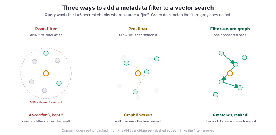
But the graph was built from vector distances alone. It knows nothing about your source field, your tenant_id, or the timestamp you want to filter on. The moment you add a predicate, the database has to reconcile a graph that ignores your filter with a result that must respect it. There are three ways to do that, and the diagram below summarizes the rest of this post.
Post-filtering: search first, filter after
The simplest implementation, and the default in more systems than you would expect, is post-filtering. The engine runs the ANN (approximate nearest neighbor) search as if there were no filter and collects its top candidates. Only then does it discard the rows that fail the predicate. Whatever survives is your result.
This works when the filter matches most of your corpus. It falls apart when the filter is selective, and you can work out why on a napkin. The pgvector docs spell it out: with the default hnsw.ef_search of 40, the index hands back 40 candidates, and “if 10% of rows match, only 4 rows will match on average” (pgvector docs). You asked for ten and got four. Narrow the filter to one percent of the corpus and you can get zero, even when plenty of good matches sit just outside the candidate window.
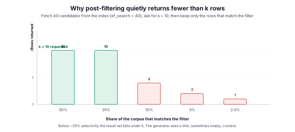
The usual first fix is to over-fetch: pull far more candidates than you need so that enough survive the filter. The snippet below sizes the candidate window from an assumed selectivity of 10%, with a safety factor on top:
# Over-fetch to compensate for a post-filter.
# If the filter keeps ~10% of rows and you want k=10,
# you need ef_search well above k just to end up near k.
FILTER_SELECTIVITY = 0.10
K = 10
SAFETY = 3
ef_search = int(K / FILTER_SELECTIVITY * SAFETY)   # ~300

rows = db.query(
    query_vector,
    ef_search=ef_search,   # widen the candidate window
    where={"source": "jira"},
    limit=K,
)
Over-fetching works until it doesn’t, for three reasons:
- You have to guess the selectivity, and it is not constant. One tenant has a million documents; another has forty.
- You pay for the worst case on every query. Set the window wide enough for the rare tenant and every query carries that latency, including the ones that never needed it.
- There is a hard ceiling. If all the matching rows sit outside the region the greedy walk explored, no candidate window can rescue the filter.
In short, over-fetching papers over the fact that the search never looked in the right place.
Pre-filtering: restrict first, then search
The opposite approach works out which rows match the filter before the vector search, usually from an inverted index or a bitmap, and confines the ANN walk to that set. Weaviate calls this pre-filtering. It builds an allow-list from its inverted index, so the graph search only ever considers matching objects. Nothing gets lost after the fact, because every candidate already passes the filter.
The catch is subtler, and it is the one people miss. An HNSW graph is navigable only because of its links. Restrict the walk to a small matching subset and you remove most of those links. The nodes you are allowed to visit may not connect to each other at all. The greedy traversal then stalls in a dead end and never reaches the true nearest neighbor: the neighbor is in the graph, but no path of edges reaches it through the allowed set.
Qdrant is blunt about this failure mode: pre-filtering “should not be used over large datasets” because it “breaks too many links in the HNSW graph, causing lower accuracy” (Qdrant). So post-filtering returns too few results, and naive pre-filtering returns the wrong ones. The same filter fails in opposite directions.
There is a saving grace. When a filter is very selective (a handful of rows out of millions), the smart move is to skip the graph and brute-force those few rows with an exact scan. Many engines do exactly this once the matching set drops below a threshold. An exact search over fifty rows is instant and, unlike the graph walk, it cannot miss. Pre-filtering is dangerous in the messy middle, not at the extremes.
Filter-aware graphs: one connected pass
The third option avoids the tradeoff. Instead of bolting the filter onto either end of a search that ignores it, it teaches the index about the filter. Distance and predicate then get evaluated together, in a single traversal that stays connected.
Qdrant’s version is a filterable HNSW. It looks at which fields you filter on and, when it builds the graph, adds extra edges so that the subgraph of matching points stays connected on its own. The greedy walk can then move from one matching node to the next without hitting a dead end, so it honors the filter without losing navigability.
One detail trips people up in practice. Qdrant builds these filter-aware edges only if the payload indexes (its indexes on metadata fields) exist before the graph is built, so the order in which you create things matters (Qdrant).
pgvector 0.8 attacks the same problem from the post-filter side, with iterative index scans. Rather than fetching one fixed batch and giving up, it keeps scanning more of the index until it has collected enough matching rows or hits a cap (pgvector docs). You turn it on per session and choose how strict the ordering has to be. The query itself stays an ordinary filtered nearest-neighbor query:
-- pgvector 0.8+: keep scanning until enough rows pass the filter
SET hnsw.iterative_scan = relaxed_order;   -- better recall, slight reorder
SET hnsw.ef_search = 100;

SELECT id, content
FROM chunks
WHERE source = 'jira'                       -- the filter
ORDER BY embedding <=> :query_vector        -- cosine distance
LIMIT 10;
The two ordering modes trade exactness for recall:
strict_orderguarantees that results come back in exact distance order.relaxed_orderlets results come back slightly out of order in exchange for better recall.
Either way, you are no longer betting a single fixed window against an unknown selectivity. The scan adapts to how rare your matching rows turn out to be.
Choosing a strategy by filter selectivity
No strategy wins everywhere, which is why every serious engine ships more than one and picks per query. The deciding factor is selectivity: the fraction of rows the filter lets through.
| Filter selectivity | Best strategy | Why |
|---|---|---|
| Matches most rows (>50%) | Post-filter | Few survivors lost; over-fetching barely needed |
| The messy middle (1 to 50%) | Filter-aware graph or iterative scan | Post-filter starves, naive pre-filter loses recall |
| Matches a handful of rows | Exact scan of the matching set | Skip the graph; brute force cannot miss and is instant |
A few practical rules hold across databases:
- Index the fields you filter on. If the engine cannot resolve a filter from an index, it falls back toward scanning. On Qdrant specifically, the filter-aware edges exist only if the payload index was there at build time.
- Know your selectivity. It decides the strategy, and it is rarely uniform. A per-tenant filter can be 0.1% for one customer and 40% for another, and the right plan differs for each.
- Measure filtered recall. Run the same queries through an exact flat search with the filter applied and compare the results. This is the same recall@k check you would do for any retrieval change. Filtered and unfiltered recall are different numbers, and the filtered one is what your users actually get.
What I would do differently
On Archi, the RAG copilot I worked on for CMS computing operations, filtering is not a feature. It is the reason the thing is usable. Operators need to scope a question to one subsystem, one logbook, or the last week of tickets, and the corpus mixes sources of wildly different sizes.
Early on, I treated the filter as a WHERE clause bolted onto retrieval and reached for over-fetching whenever results looked thin. That is the move I would skip now. Over-fetching hid the symptom but left the real questions unanswered: how selective is this filter, and is my engine pre-filtering, post-filtering, or neither? Meanwhile, recall on the narrow, high-value queries stayed quietly bad.
The better instinct is to decide the filtering strategy up front, from the selectivity you expect, rather than discovering it from a starved result set in production. Treat a filtered vector search as its own thing with its own recall number, not as unfiltered search with a predicate stapled on. The index does not see your WHERE clause the way you do, and the whole game is closing that gap on purpose instead of by accident.
The diagrams in this post were generated for it. Nearest-neighbor illustration style adapted from my earlier HNSW walkthrough.