Binary Quantization for Vector Search

The bill for a vector index is mostly RAM, and RAM is the resource you notice last and pay for first. A modern embedding model hands you a 1024-dimensional float32 vector per chunk. That is 4 kilobytes each. A million chunks is four gigabytes of raw vectors, before you count the graph edges an HNSW index stacks on top. Approximate search wants all of it resident, because a graph walk that pages off disk is not fast in any useful sense. At ten million chunks, you are provisioning a node around the embeddings rather than the workload.

Binary quantization attacks that number directly. Keep one bit per dimension instead of thirty-two, and the same vectors shrink by a factor of 32. The catch is obvious: throwing away that much precision should wreck your results. It mostly does not, and the reason it does not is worth understanding before you turn it on.

This post is for engineers who already run a RAG (retrieval-augmented generation) or semantic-search system and have watched the memory footprint climb. Binary quantization is a compression option that is simpler than product quantization and needs no training step. I will cover what the transform actually is, why Hamming distance makes it fast, the rescoring pass that buys the recall back, and where it quietly falls apart.

The whole transform is one comparison

Binary quantization keeps the sign of each dimension and discards the magnitude. A value above zero becomes a 1; everything else becomes a 0. That is the entire encoder. There is no codebook to train, no centroids to fit, and nothing to keep in sync with the model. You run it once when you index, and again on each query.

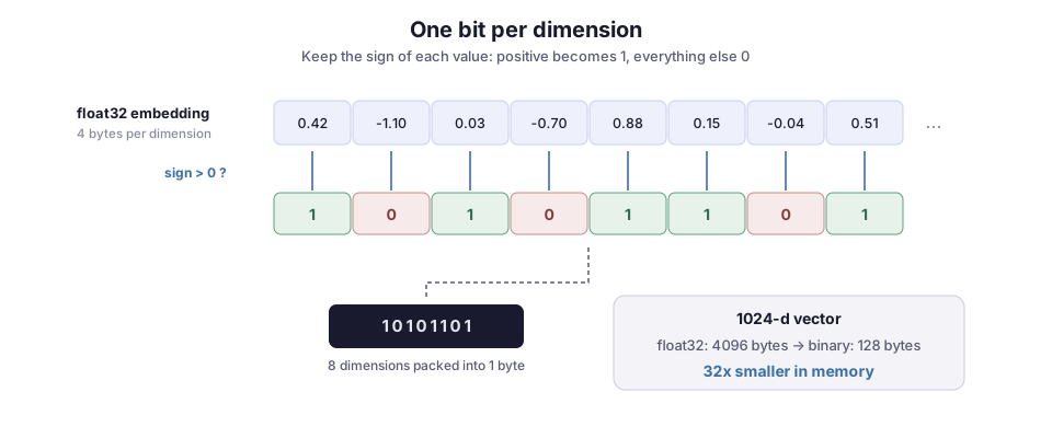
Eight bits pack into a byte, so a 1024-dimensional vector collapses from 4096 bytes to 128.

What is easy to miss is that this only works because of how modern embeddings are shaped. Sentence and document models produce high-dimensional vectors, where meaning is spread across hundreds of coordinates. Most inference stacks also L2-normalize the output (scale each vector to length 1), so every vector sits on the unit sphere. On the sphere, the sign pattern across dimensions carries most of the angular information, and cosine similarity is a measure of angle.

That is the load-bearing assumption. Binarizing a low-dimensional or unnormalized vector destroys far more. This is the first failure mode, and the one people trip on when they try it on 384-dimensional embeddings and get noise back.

Hamming distance: why it is fast, not just small

Compression alone would be reason enough, but the bigger win is the distance function. To compare two binary vectors, you count the positions where their bits differ. That count is the Hamming distance. In hardware it is an XOR (which marks the bits that differ) followed by a population count (which counts them). POPCNT is a single CPU instruction that chews through 64 dimensions per operation. There is no floating-point multiply and no accumulation, just integer ops the processor already loves.

The practical effect is that a scan over binary vectors runs far faster than the equivalent float32 dot products, on top of touching 32 times less memory. When Cohere shipped binary support for their embeddings, they reported roughly a 40x speedup on the distance computation alongside the memory reduction.

Here are the encoder and the distance in NumPy, which is enough to see the mechanics. binarize sets a bit for every positive value and packs the bits into bytes. hamming XORs the query against every stored vector and counts the bits that differ:

import numpy as np

def binarize(vectors: np.ndarray) -> np.ndarray:
    # vectors: (n, d) float32. One bit per dimension: 1 if > 0 else 0.
    bits = (vectors > 0).astype(np.uint8)
    return np.packbits(bits, axis=1)          # (n, d/8) uint8

def hamming(query_bits: np.ndarray, corpus_bits: np.ndarray) -> np.ndarray:
    # query_bits: (d/8,)  corpus_bits: (n, d/8)
    xor = np.bitwise_xor(corpus_bits, query_bits)
    return np.unpackbits(xor, axis=1).sum(axis=1)

np.packbits does the bit packing (docs). A real system leans on a library like Faiss, which has IndexBinaryFlat and IndexBinaryHNSW and uses hardware popcount under the hood. The NumPy version is for reading, not for a million-vector corpus.

Rescoring is what makes it usable

If you stop at Hamming distance, recall drops enough to notice. The sign pattern is a good approximation of direction, not an exact one. So the top-k it returns is close to the true top-k, but shuffled and missing a few. For a lot of production work, “close but shuffled” is a bug.

The fix is a two-stage search, and it is the reason binary quantization is practical rather than a curiosity:

1. Use the binary index to pull a shortlist far larger than what you actually want.
2. Rescore that shortlist with the full-precision vectors, and keep the real top-k.

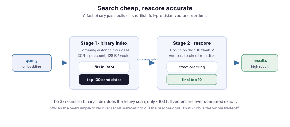
Concretely: to get the top 10, retrieve the top 100 or 200 by Hamming distance, compute exact cosine on just those against their float32 vectors, and re-sort. Only the binary index has to live in memory. The full vectors sit on disk or in a cheaper tier, and get fetched by ID for the handful of candidates that survive stage one. So you keep the 32x memory saving on the part that has to be resident, and pay for full precision on a hundred vectors instead of a million.

The search function below puts both stages together, with a shortlist of k * oversample candidates:

def search(query, corpus_bits, corpus_full, k=10, oversample=10):
    q_bits = binarize(query[None, :])[0]
    dists = hamming(q_bits, corpus_bits)

    # stage 1: cheap binary shortlist, oversampled
    cand = np.argpartition(dists, k * oversample)[: k * oversample]

    # stage 2: exact cosine on the shortlist's float32 vectors
    scores = corpus_full[cand] @ query          # vectors are normalized
    return cand[np.argsort(-scores)[:k]]

The oversample factor is the one knob that matters. Retrieve 10x the vectors you need and rescore, and the reported recall on large embedding models lands around 96% of exact float search, while the index is a fraction of the size. Hugging Face’s write-up has the benchmarks across several models. Widen the multiplier and recall climbs toward exact, at the cost of a bigger rescore. Narrow it and you save compute, but start dropping real results.

There is no single right value. It depends on your embedding model and on how much recall loss your users would actually feel. Measure it against a labeled set rather than guessing, the same way you would when tuning any retrieval component.

Asymmetric search when you need more recall

There is a middle option between full binary and full float: binarize the stored vectors, but keep the query in float32. To compare them, treat each stored bit as +1 or -1 and take a dot product with the float query. The corpus still costs one bit per dimension, so the memory saving holds. But the query side carries more signal into the comparison, so recall improves over pure binary-to-binary search. You pay for it with a slower scan, because you are back to arithmetic instead of popcount.

It is a reasonable default when a single binary pass loses too much and you would rather not oversample as aggressively. Qdrant’s quantization guide documents this asymmetric mode and the oversampling settings around it, if you want a system that already implements both.

Where it bites

The failures are consistent, and mostly about knowing when not to reach for it.

Small dimensions lose too much. Binary quantization needs the redundancy of a high-dimensional space to survive dropping the magnitude. At 1024 or 1536 dimensions it holds up. At 384, the sign pattern is too coarse, and recall falls off a cliff even with rescoring. Check your model’s output width before assuming this applies.

Not every model binarizes well. The technique relies on the embedding geometry being cooperative, and models differ. Some vendors publish binary recall numbers because they tested it and it works; others do not, and you should not assume. Run your own recall check against exact search on a real query set before trusting it. “It compiled and returned results” is not the same as “it returned the right results.”

The corpus has to be big enough to matter. All of this is overhead you are adding to save memory. Under a few hundred thousand vectors, exact float search is fine, and probably faster end to end once you count the rescore fetch. Binary quantization earns its complexity at scale, not on a side project.

Rescoring needs the float vectors somewhere. You are not deleting the full-precision embeddings; you are demoting them off the hot path. They still have to be fetchable by ID with low latency, or stage two becomes the bottleneck the whole design was meant to avoid. If your storage tier makes random reads slow, this is where it shows up.

What I would reach for first

If I were shrinking an index today, binary quantization with rescoring is the first thing I would try, ahead of product quantization. The reason is simple: there is no codebook to train, and nothing to retrain when the corpus drifts. The encoder is a sign check. The failure modes are legible. And the one tuning parameter, the oversample factor, maps cleanly onto a recall-versus-cost curve you can plot and defend.

This is the kind of tradeoff that decides whether a retrieval system stays affordable as its corpus grows. On Archi, the RAG copilot I built for CMS operations at CERN, the document and log corpus only goes one direction. There, the difference between float32 and binary vectors is the difference between one index node and several. It is the same instinct behind the rest of the operations tooling I maintain: pick the representation that keeps the system cheap to run a year from now, not just the one that is easy to stand up this week.

Compression is a design choice about what has to fit in memory, and it pays to make it early rather than bolt it on once the index no longer fits. Which embedding model you start from constrains all of it, because the model’s dimensionality and geometry decide whether binary quantization is a free win or a non-starter.

Diagrams by M. Hassan Ahmed, released under CC0. No external image was used for this post; the figures are original work by the author.