Measuring RAG Retrieval Quality: recall@k, MRR

You swap the embedding model, add a keyword branch, bolt on a reranker, and the answers feel better, so you ship it. Two weeks later someone asks a question the old pipeline handled fine, and the new one whiffs. You have no way to tell whether you actually improved retrieval or just moved the failures somewhere you weren’t looking. I did this for longer than I’d like to admit: tuning a retrieval pipeline by reading a handful of outputs and trusting my gut.

The fix is boring, and it works. Freeze a set of questions with known-good answers, run each candidate pipeline against it, and compute a few numbers. This post is for engineers who already have a working RAG (retrieval-augmented generation) system and keep changing the retrieval layer without a way to score the change. I’ll cover how to build the evaluation set, the three metrics worth computing, a small script that computes them, and where the numbers lie to you.

Grade retrieval separately from generation

A RAG answer can be wrong for two very different reasons:

• Retrieval failed. The retriever never surfaced the right chunk, so the model was answering from nothing.
• Generation failed. Retrieval found the right chunk, and the model still botched the summary.

These need different fixes, and lumping them into one “is the answer good” judgment hides which one you have.

This post is only about the first half. Given a query, did the retriever return the chunks that actually contain the answer, and were they near the top? That is a ranking problem, with decades of established measurement behind it from the information retrieval world. Grading the generated text is a separate exercise. If you mix the two, a retrieval regression can hide behind a model that happens to paper over it. Score retrieval on its own first.

Build a golden set of queries and relevant chunks

The golden set is a list of queries, each paired with the IDs of the chunks that count as relevant answers. Everything downstream is just arithmetic on top of it, so this is the part that decides whether your evaluation means anything. In code, it is a mapping from query ID to a set of chunk IDs:

# golden.py: ground truth mapping query id -> set of relevant chunk ids
GOLDEN = {
    "q_fnal_transfer": {"chunk_8842", "chunk_5507"},
    "q_pileup_config": {"chunk_1290"},
    "q_site_blacklist": {"chunk_0774", "chunk_0775", "chunk_3301"},
    # ... 50 to 200 of these
}

There are two honest ways to build it:

• Mine your own logs. This is the best source: real questions people asked, each paired with the chunk that actually answered it, confirmed by hand. It’s slow and it’s worth it, because those queries carry the vocabulary and the weird edge cases your synthetic ones never will.
• Generate questions with an LLM. Sample real chunks and have an LLM write a question each one answers. That gets you volume, but watch for circularity. If the same embedding model writes the questions and does the retrieval, you’re partly grading the model against its own phrasing, and the score comes out flattering.

I mix both, and I keep the log-derived queries as the set I actually trust.

Fifty queries is enough to catch a real regression, and a couple hundred makes the number stop jumping around between runs. Also keep the set out of anything you tune on. A golden set you’ve optimized against is just a training set with a nicer name, and it stops predicting how the pipeline behaves on questions you haven’t seen.

Three metrics: recall@k, MRR, and nDCG

For each query, the retriever returns a ranked list of chunk IDs. All three metrics are functions of that list and the relevant set from the golden data. They answer different questions, so compute all three.

recall@k asks did the right chunks show up in the top k at all? It’s the fraction of the relevant chunks that landed in the top k results. This is the metric that maps most directly to RAG, because a chunk the model never sees can’t help it. If recall@10 is low, no amount of reranking saves you; the answer isn’t in the candidate set.

MRR (Mean Reciprocal Rank) asks how high was the first good hit? For each query you take 1 / rank of the first relevant chunk, then average across queries. It rewards getting one right answer to the top and ignores the rest. That matches how a context window fills up: the first relevant chunk at position 1 is worth a lot more than the same chunk at position 9.

nDCG@k (Normalized Discounted Cumulative Gain) asks is the whole ordering any good? It gives every relevant chunk in the top k a credit that shrinks the lower it ranks, and sums those credits. Then it divides by the score of the perfect ordering, so the result lands between 0 and 1. It’s the one to watch when several chunks are relevant and you care about the shape of the ranking, not just the first hit.

The three functions below compute each metric for a single query:

import math

def recall_at_k(retrieved, relevant, k):
    hits = sum(1 for doc in retrieved[:k] if doc in relevant)
    return hits / len(relevant)

def reciprocal_rank(retrieved, relevant):
    for rank, doc in enumerate(retrieved, start=1):
        if doc in relevant:
            return 1 / rank
    return 0.0

def ndcg_at_k(retrieved, relevant, k):
    dcg = sum(1 / math.log2(rank + 1)
              for rank, doc in enumerate(retrieved[:k], start=1)
              if doc in relevant)
    ideal_hits = min(len(relevant), k)
    idcg = sum(1 / math.log2(rank + 1) for rank in range(1, ideal_hits + 1))
    return dcg / idcg if idcg else 0.0

The log2(rank + 1) in nDCG is the discount: rank 1 divides by 1, rank 3 by 2, rank 7 by 3. Later positions count for progressively less, which is the whole point. IDCG (the ideal DCG) is the same sum computed as if every relevant chunk were stacked at the top. Dividing by it means a query where a perfect retriever could only fit three relevant chunks in the top k isn’t unfairly punished against one with a single answer.

Compare pipelines with a small runner

A run is each query’s ranked list from one pipeline. Given a run and the golden set, averaging the per-query scores is the whole evaluation. The loop at the bottom scores three configurations against the same golden set: dense, hybrid, and hybrid plus a reranker.

def evaluate(run, golden, k=10):
    rows = []
    for qid, relevant in golden.items():
        retrieved = run[qid]                       # ranked chunk ids
        rows.append((
            recall_at_k(retrieved, relevant, k),
            reciprocal_rank(retrieved, relevant),
            ndcg_at_k(retrieved, relevant, k),
        ))
    n = len(rows)
    return {
        f"recall@{k}": sum(r[0] for r in rows) / n,
        "MRR":         sum(r[1] for r in rows) / n,
        f"nDCG@{k}":   sum(r[2] for r in rows) / n,
    }

for name, run in [("dense", run_dense),
                  ("hybrid", run_hybrid),
                  ("hybrid+rerank", run_rerank)]:
    print(name, evaluate(run, GOLDEN, k=10))

Run it once per candidate configuration, and you get the comparison the gut check never could. The diagram below shows the whole workflow: same golden set, same queries, swap only the retriever, and read the numbers.

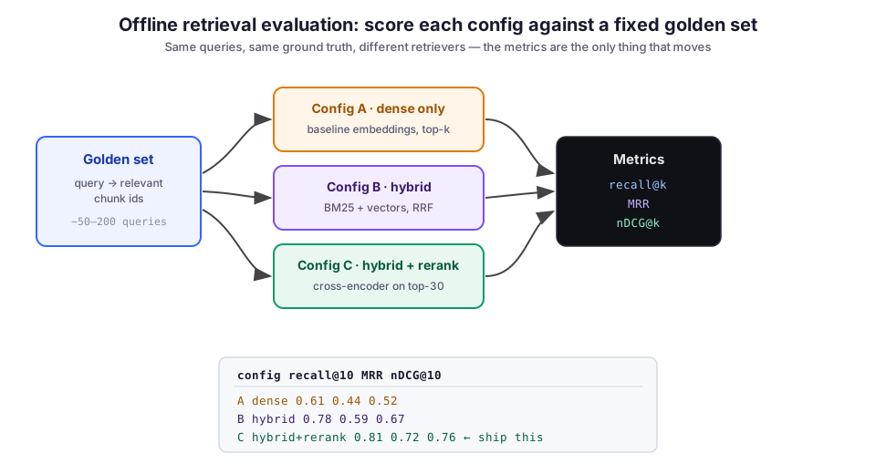
The point of a table like that isn’t the absolute values, which depend entirely on how you built the golden set. It’s the deltas between rows:

• Hybrid lifting recall@10 from 0.61 to 0.78 means the keyword branch is pulling in relevant chunks that dense retrieval missed.
• The reranker barely moving recall but jumping MRR from 0.59 to 0.72 is exactly its signature. It doesn’t find new chunks; it reorders the ones you have so the good one lands first.

Reading the deltas this way tells you which knob did the work. I wrote up that exact pipeline, hybrid search with BM25 and vectors plus a cross-encoder, in a separate post; this evaluation is how I decided it was worth keeping.

Write the metric functions once to understand them, then reach for a real library in production. ranx and ir_measures implement these and a dozen more with the edge cases handled. BEIR gives you standard datasets to sanity-check a retriever against, and Ragas covers the generation half once you’ve nailed retrieval.

Where the numbers lie

A metric is only as trustworthy as the setup behind it. These are the ways the setup goes wrong.

A tiny golden set that swings every run. With 20 queries, one flaky question flips a metric by five points, and you end up chasing noise. If the number won’t sit still between identical runs, add queries before you trust any delta.

Grading generation and blaming retrieval. If your eval reads the final answer instead of the retrieved IDs, a strong model hides a weak retriever and a weak model buries a strong one. Score the ranked list of chunk IDs directly, before the LLM touches them.

k set to what you retrieve instead of what you use. If you feed the model the top 5 chunks, recall@20 is a comforting number that doesn’t matter, because chunks 6 through 20 never reach the context. Measure at the k you actually pass downstream.

Incomplete relevance labels. Mark only one chunk relevant when three answer the question, and the retriever gets “penalized” for surfacing a genuinely good chunk you forgot to label; every unlabeled relevant chunk drags your scores down for no real reason. When a config scores worse than it feels, spot-check whether it found good chunks your golden set never credited. This one bit me on a corpus where the same fact lived in several near-duplicate documents.

What I’d do differently

I built the golden set too late, after I’d already made three retrieval changes I couldn’t untangle. If I’d frozen 50 queries before touching anything, each change would have been one clean line in a table instead of a guess. Build the eval first, even a rough one, because a rough measurement beats a confident feeling.

I also over-indexed on a single metric early on. I stared at recall while MRR quietly told me the right chunk was consistently landing at rank 8. Recall says the answer is in there; MRR and nDCG say where. In RAG the context window is small and position matters, so you need both readings or you optimize the wrong half.

Where I use this

Retrieval evaluation is how I kept Archi, the RAG copilot I worked on for CMS computing operations at CERN, from silently regressing every time I touched the pipeline. Operators ask about specific site names, error codes, and ticket IDs. A change that helps the vague questions can quietly break the exact ones, and only a golden set built from real operator queries catches that trade before it ships.

The same eval told me whether incremental re-indexing had drifted the results after a partial rebuild. It also settled the retriever choices on ARGRAG, the enterprise-document RAG system my teammate and I built for the Argusa AI Challenge. A pipeline you can’t measure is a pipeline you’re tuning by vibes, and vibes don’t survive contact with the query you didn’t think to try.

Image credit: diagrams by M. Hassan Ahmed, created for this post and released under CC0. Example queries reference the Archi project.