Product Quantization for Vector Search

The HNSW post ended on a bill I did not pay. HNSW makes the search fast by walking a graph in a handful of hops instead of scanning the whole corpus. But it still keeps every embedding resident in memory as raw float32. On a small index nobody notices. On a corpus where every log line, ticket, and doc page becomes a chunk, the vectors themselves stop fitting in the box. They run out of room before query latency ever becomes a problem.

This post is about shrinking the vectors, not the search over them. The technique is product quantization (PQ), first described by Jégou, Douze, and Schmid in 2011. It is what sits underneath the “compressed” index types in FAISS, Milvus, and Qdrant. The post is for engineers who already have vector search working, have watched the memory number climb, and want to know what the index is doing when it trades exactness for room to grow.

The problem is memory, not speed

Do the arithmetic once and it sticks. A million chunks at 768 dimensions, four bytes per dimension, is 1e6 × 768 × 4 ≈ 3 GB of vectors alone. The HNSW graph adds more on top, because every node stores a list of neighbor ids. Push the corpus to ten million and you are near 30 GB.

All of it has to stay resident. Approximate nearest neighbor search is random access by nature, so there is no hot working set to page in and out. You can shard across machines, but each shard still holds its slice in RAM.

So the question changes. HNSW answered “how do I look at fewer vectors?” Product quantization answers a different one: “how do I make each vector smaller?” The goal is small enough that the whole index stays in memory, instead of spilling to disk or onto a bigger, pricier instance.

Scalar quantization gets you 4x, then stops

The first move most people make is scalar quantization: map each float32 dimension to an int8, one byte instead of four. That is a clean 4x, it is cheap, and recall barely moves for most embedding models, which is why several vector databases now default to it. But it treats every dimension on its own, so it bottoms out at one byte per dimension. To go further you have to stop quantizing dimensions independently, and that is exactly the door PQ walks through.

The idea: quantize chunks of the vector

PQ encodes a vector in three steps:

1. Split the D-dimensional vector into m contiguous sub-vectors.
2. In each subspace, run k-means on a sample of your data to learn a small codebook of k centroids (representative points for that slice). Pick k = 256, and a centroid id fits in a single byte.
3. Replace each sub-vector with the id of its nearest centroid.

The whole vector is now m bytes.

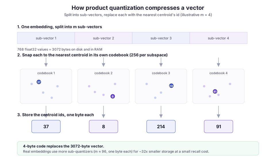
The word “product” is the interesting part. With m codebooks of 256 entries each, you can represent 256^m distinct vectors: the Cartesian product of the per-subspace choices. Yet you only ever store m × 256 centroids. That combinatorial reach from a tiny table is the whole trick.

The compression follows from m. Take a 768-dim embedding, which is 3072 bytes as raw floats. Split it into m = 96 sub-vectors of 8 dimensions each, at one byte per sub-quantizer, and you land at 96 bytes: about 32x smaller. Drop to m = 48 and you get 48 bytes and 64x, with more error, because each byte now has to summarize a wider slice of the vector. The diagram uses m = 4 so the codebooks are legible. In practice the knobs are m (how many pieces) and nbits (how many centroids per piece, set as bits per code; almost always 8).

Computing distances without decompressing

This is the part that makes PQ fast at query time and not just small on disk: you never rebuild the vector. The method is asymmetric distance computation (ADC):

1. Keep the query at full precision, and split it the same way.
2. For each subspace, precompute a small table of distances from the query’s sub-vector to all 256 centroids of that codebook. That is an m × 256 table, built once per query.
3. The distance from the query to any stored code is now a sum of m lookups. For each sub-quantizer, use the code’s stored byte as the index, read one cell, and add the cells up.

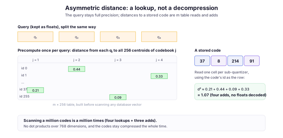
With the diagram’s m = 4, scanning a million codes becomes a million rounds of “four reads and three adds.” There are no 768-dimension dot products and no decompression anywhere in the loop.

There is also a symmetric variant that quantizes the query too. It lets you reuse tables across queries, but it folds the query’s own quantization error into every distance. “Asymmetric” keeps that error out of the estimate, so ADC is the default worth reaching for.

PQ alone still scans everything, so pair it with IVF

One honest caveat: PQ shrinks the vectors, but by itself it does not reduce how many you compare against. A million lookups is fast, but it is still O(N). So in practice PQ rides underneath a coarse index that narrows the candidate set first.

The classic pairing is an inverted file index, IVF:

• A coarse k-means partitions the space into cells.
• The query probes only the nprobe nearest cells.
• PQ encodes the residual (the vector minus its cell’s centroid), which has smaller magnitude and therefore quantizes more accurately.

That combination, IVF-PQ, is the workhorse of large FAISS indexes. It shows up in the index factory strings people paste around, like IVF4096,PQ96. You can also put PQ codes under an HNSW graph instead of IVF: same division of labor, different coarse structure.

Where it bites

The happy path is short. The engineering is in the edges, and PQ has a few sharp ones.

Recall drops, and you feel it at the top of the list. Approximate distances reorder near-ties, so the true nearest neighbor sometimes comes back ranked third. The standard fix is a two-stage read: pull a larger shortlist with PQ, then rerank it with exact full-precision vectors. That only works if you kept the full vectors somewhere. FAISS’s IndexRefineFlat does exactly this: it buys the memory back, but only for the shortlist, not the whole corpus. Measure recall against a flat baseline before and after. The whole point of PQ is the trade (how much recall you give up for the memory you save), and you cannot judge that trade without the number.

Codebooks are trained, so they go stale. Those centroids were learned by k-means from a sample of your embeddings. Swap the embedding model, or let the corpus drift into a new domain, and the codebooks no longer describe the vectors you are storing. Encoding error then climbs quietly. Retraining means re-encoding everything, which runs straight into the incremental indexing tradeoffs: you cannot just append; you have to rebuild.

Variance is uneven across dimensions, and naive splits waste bits. Chop a vector into contiguous slices and one sub-quantizer may get all the high-variance dimensions while another gets nearly constant ones. Both spend the same 256 centroids on very different amounts of information. Optimized product quantization (OPQ), from Ge, He, Ke, and Sun, learns a rotation first, so variance spreads evenly across subspaces before quantizing. It is usually close to a free recall bump, and FAISS exposes it as an OPQ pre-transform you prepend to the index string.

The metric has to match. Textbook PQ assumes Euclidean (L2) distance. Most modern text embeddings are compared with cosine or inner product, so normalize the vectors first. Otherwise, the geometry the codebooks were built around is not the geometry you are querying in.

Small corpora do not need it. If the raw vectors fit in RAM (a few hundred thousand 768-dim vectors is one to two gigabytes), PQ only adds error for no real saving. It earns its place when memory is the binding constraint, not as a reflex.

What I would reach for, in order

The order of moves as an index grows is fairly settled:

1. Keep flat or HNSW with full float32 while it fits.
2. Reach for scalar int8 when you want a cheap 4x and can spare a little recall.
3. Move to IVF-PQ, or HNSW over PQ codes, once you are genuinely memory-bound in the millions. When you do, add OPQ and keep an exact-rerank step for the shortlist.

At every step, hold the flat baseline’s recall@k (how many of the true top k the index returns) next to the compressed index’s. That gap is the only thing that tells you whether the memory you saved cost you answers.

For Archi, the retrieval copilot I worked on for CMS computing operations at CERN, this is not a hypothetical. The knowledge base has no natural ceiling: every new logbook entry and ticket is another chunk. It is the vectors, not the graph traversal, that threaten to price the index out of the memory it runs in. PQ is the lever that keeps a growing dense index resident. It sits quietly under the dense half of hybrid search, and the whole point is that once the recall math checks out, nobody upstream has to think about it again.

---

Diagrams by M. Hassan Ahmed, released under CC0. No external image was used for this post; the figures are original work by the author.