How HNSW Vector Search Actually Works
Every RAG stack leans on HNSW but treats it as a black box. Here is how the layered graph index finds nearest neighbors fast, and the knobs that matter.

Every RAG (retrieval-augmented generation) post I have written so far ends up calling the same function: give me the k chunks whose embeddings are closest to this query. Chunking decides what goes in the index, hybrid search decides how you query it, and reranking decides what survives into the prompt. In the middle of all that is one line, index.search(query_vector, k=50), and I have been treating it as free.
It is not free, and the thing making it fast almost certainly has four letters: HNSW. If you use pgvector, Qdrant, Weaviate, Milvus, FAISS, or OpenSearch’s k-NN plugin, HNSW is the default index behind that search call.
This post is for engineers who have vector search working and want to know what the index is actually doing when:
- recall (the share of the true nearest neighbors the search returns) drops;
- memory blows up;
- a config value copied off a blog post turns out to matter.
I will cover the exact-search problem HNSW dodges, how its layered graph routes a query, the three parameters worth understanding, and the failure modes that bite in production.
The problem: exact nearest-neighbor search does not scale
Start with the naive version. You have a query vector and a corpus of N document vectors, each maybe 768 or 1536 dimensions. The exact answer is a linear scan: compute the distance from the query to every one of the N vectors, sort, and take the top k. This is called a flat index, and it is genuinely exact.
It is also O(N) per query. For a few thousand vectors that is fine, and you should not reach for anything cleverer. But in the corpus behind a real copilot, every log line, ticket, and doc page becomes a chunk. N is in the millions, and a full scan on every keystroke is not a latency you can pay. Worse, the curse of dimensionality breaks the usual shortcuts. The tree structures that speed up low-dimensional nearest-neighbor search (kd-trees and friends) collapse back toward a full scan once you are in hundreds of dimensions.
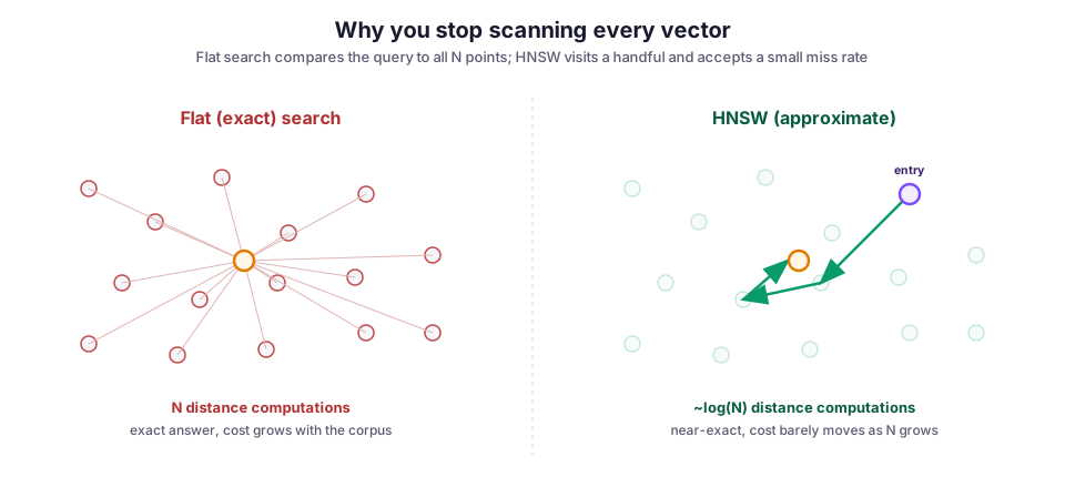
So you give up exactness. Approximate nearest neighbor (ANN) search accepts that it will occasionally miss the true closest vector. In exchange, query cost grows like log(N) instead of N. Every ANN method answers the same question in its own way: how do you visit a handful of promising vectors instead of all of them, without a tree? HNSW answers it with a graph.
The idea: a navigable small-world graph
HNSW stands for Hierarchical Navigable Small World. It comes from Malkov and Yashunin’s 2016 paper (later in IEEE TPAMI). The name holds two ideas, and together they are the whole trick, so it is worth pulling them apart.
A navigable small world graph is one where every node has a few short-range links to near neighbors and a few long-range links to far-away nodes. That mix is what makes a small-world network. The short links keep each neighborhood connected, and the rare long links mean any two nodes are only a few hops apart. Drop a query into such a graph and keep walking to whichever neighbor is closest to the query, and you reach the query’s neighborhood quickly. That greedy walk is the search.
The catch with a single flat small-world graph is that the greedy walk can be slow to cover distance. Near the start you want huge strides, but the graph only offers whatever links the current node happens to have. That is what the hierarchy fixes.
How the layers work
HNSW stacks several graphs on top of each other. When a vector is inserted, it is assigned a top layer drawn from an exponentially decaying distribution. So most vectors live only on layer 0, a smaller fraction also reach layer 1, fewer still reach layer 2, and so on. Layer 0 contains every vector, and each layer above is a sparse sample of the one below. The exponential decay is the same probabilistic idea behind a skip list, lifted from one dimension into a graph.
Search runs top-down:
- Start at a single entry point in the top, sparsest layer.
- Greedily hop to the neighbor closest to the query until no neighbor is closer. Because this layer is sparse, each hop covers a lot of ground.
- Drop straight down to the same node in the next layer and repeat, now with denser links and shorter hops.
- At layer 0, do the same greedy walk but keep a candidate list of the best nodes seen, and return the top
k.
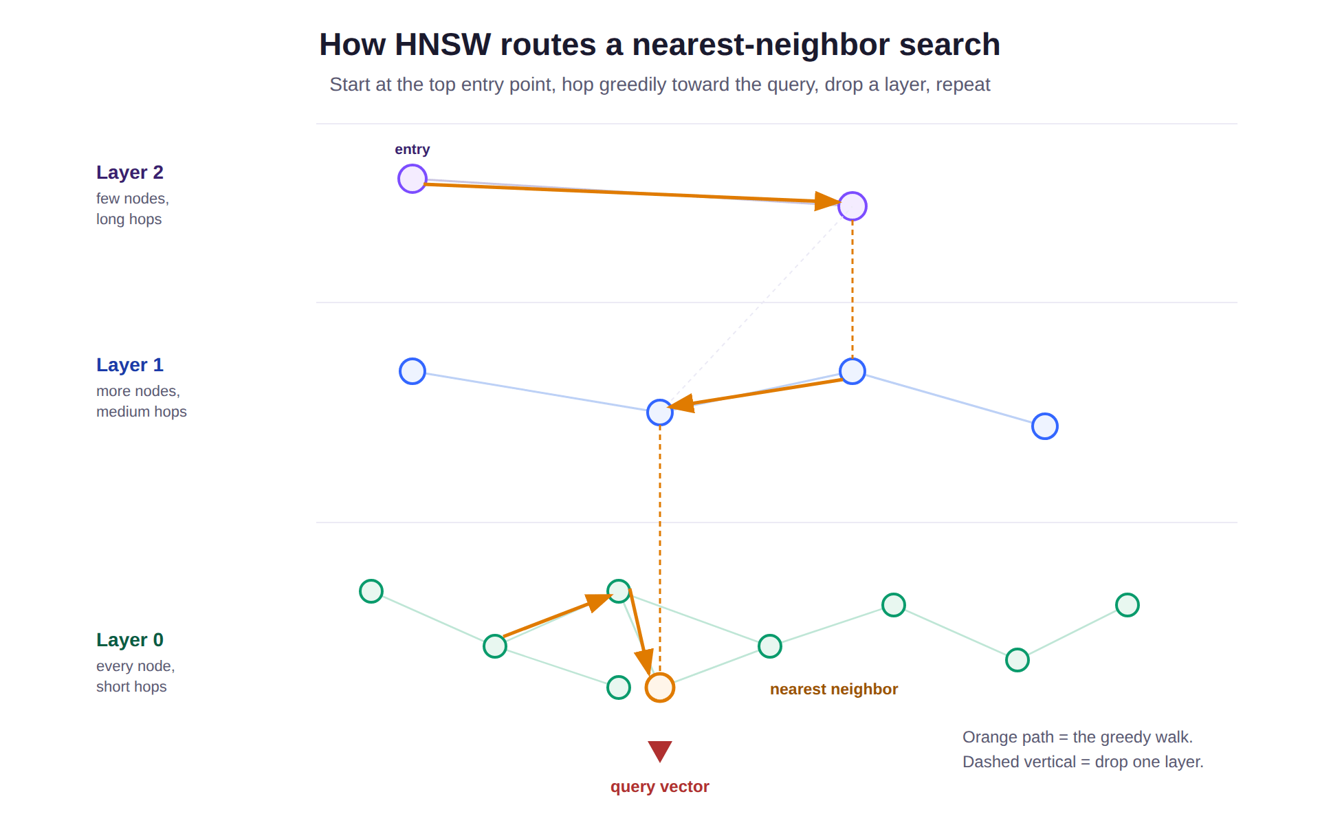
The top layers are a coarse approach that gets you into the right region in a few long hops. The bottom layer is the fine-grained search that finds the actual neighbors. That is why the cost scales with log(N): you are descending a hierarchy, not scanning a list.
The three parameters that matter
Almost every HNSW implementation exposes the same three knobs under slightly different names, and understanding them is most of what you need to tune an index. The values below are pgvector’s defaults, but the meanings carry across FAISS, OpenSearch, and the rest.
m: links per node (build time). This sets how many neighbors each node keeps on the graph. Higher m means a denser, better-connected graph with higher recall. The cost is more memory (every link is stored) and slower builds. pgvector defaults to 16; the useful range is roughly 5 to 48. This is the parameter that most directly sets your memory footprint, because the graph edges live in RAM alongside the vectors.
ef_construction: search width while building (build time). To insert a node, HNSW runs a search to find its neighbors, and ef_construction sets how wide that search is. Bigger means better neighbor choices and a higher-quality graph, at the cost of slower inserts. pgvector defaults to 64. You pay this once, at build time, so it is usually worth setting generously.
ef_search: search width at query time (query time). This is the size of the candidate list the greedy walk keeps at layer 0. It is the runtime accuracy-versus-latency dial, and the one you will actually reach for. Raise it and the walk explores more of the graph: recall climbs toward the exact answer, and latency climbs with it.
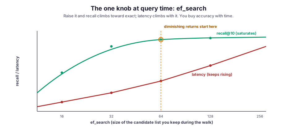
The shape of that trade is the important part. Recall saturates: past some ef_search, you pay real latency for accuracy gains too small to notice. Latency does not saturate. So the job is to find the elbow of the curve. The only honest way to find it is to measure recall against an exact flat search on your own data, which comes up again in the failure modes below.
In practice: pgvector and FAISS
If your vectors already live in Postgres, pgvector is the least-friction option, and the parameters map straight onto the section above. In the example, the build-time knobs go on the index, ef_search is a session setting, and the query orders results by cosine distance:
-- build-time knobs live on the index
CREATE INDEX ON chunks
  USING hnsw (embedding vector_cosine_ops)
  WITH (m = 16, ef_construction = 64);

-- query-time knob is a session GUC
SET hnsw.ef_search = 100;

SELECT id, content
FROM chunks
ORDER BY embedding <=> :query_vector   -- <=> is cosine distance
LIMIT 50;
One detail deserves attention: the operator class, here vector_cosine_ops, has to match the distance your embeddings were made for. Suppose your embedding model produces vectors meant for cosine similarity, and you build the index with L2 distance (vector_l2_ops). The index is “working,” but it is quietly ranking by the wrong metric. That mismatch stays invisible until you measure retrieval quality.
For a standalone index, FAISS exposes the same graph directly. Note that the positional 16 passed to the constructor is m:
import faiss

d = 768                          # embedding dimension
index = faiss.IndexHNSWFlat(d, 16)      # 16 == m
index.hnsw.efConstruction = 64
index.add(doc_vectors)                  # np.float32, shape (N, d)

index.hnsw.efSearch = 100               # the query-time dial
distances, ids = index.search(query_vectors, k=50)
Same three numbers, same meanings. FAISS’s own guidance on choosing an index is a good second read once you are deciding between HNSW and the quantized variants for a large corpus.
Failure modes
Deletes do not really delete. HNSW is built for insert-and-search, not churn. Most implementations handle a delete by tombstoning the node (marking it deleted while leaving it in the graph) rather than removing it. Unpicking a well-connected node and rewiring its neighbors is expensive. In a corpus that updates often, tombstones accumulate, the graph degrades, and recall drifts down. I hit exactly this tension when I wrote about keeping a RAG index fresh. The clean answer is often a periodic rebuild rather than an endless stream of in-place deletes.
The index is a memory cost, not just a disk cost. HNSW keeps the graph, and usually the vectors, in RAM to hit its latency numbers. A denser graph (higher m) takes more memory. It is easy to size a box for the raw vectors, forget the graph edges on top, and then watch the process get killed under load. Budget for both before you pick m.
“Recall” you never measured. ANN is approximate by definition. The amount of approximation is a config value you chose, sometimes by accident, by taking a library default. The only way to know your real recall is to run a sample of queries through both the HNSW index and an exact flat search, then compare the results. This is the same golden-set discipline I described in measuring RAG retrieval quality. Your ef_search matters because it silently sets the recall those metrics report.
Tuning against the wrong stage. If the right chunk is missing from your results, the index is only one of the suspects. Bad chunking can mean the answer was never a clean vector to begin with. A metric mismatch can mean the graph is ranking by the wrong distance. Before you turn ef_search up, confirm the vector is even in the corpus and that a flat search finds it. An ANN index can only fail to find what an exact search would have found. If the exact search misses it too, the bug is upstream.
What I would do differently
My mistake was treating the vector index as infrastructure that either works or does not, and reaching for it as the first knob when retrieval quality dropped. The index is a dial, not a switch, and its default position was chosen by a library author who had never seen my data. Now, before the index goes near production, I:
- build a small golden set of query-to-expected-chunk pairs;
- measure recall against a flat search;
- only then decide whether the default
ef_searchis fine, or whether I am silently dropping a tenth of the right answers.
Doing that first turns HNSW from a black box into one more measurable stage in the pipeline.
Why it matters: approximation is a number you set
HNSW is the quiet layer under every RAG post I have written: the thing that makes “find the nearest chunks” cheap enough to do on every request. It is the retrieval engine inside Archi, the RAG copilot I worked on for CMS computing operations at CERN. It is the reason a query against millions of indexed log lines and tickets comes back in milliseconds instead of scanning the lot.
The layered graph is a genuinely elegant piece of engineering. But the part that matters for a production system is smaller and less glamorous. The index is approximate, the amount of approximation is a number you set, and you do not know that number until you measure it. Once you treat the index as a stage you can score, the same way you score chunking and reranking, it stops being a black box and starts being tunable.
Diagrams by M. Hassan Ahmed, released under CC0. Image credit: original work by the author.