IVF Vector Search: Search Fewer Vectors
Brute-force vector search compares every embedding. How an IVF index partitions vectors into cells, probes only the nearest, and where the nprobe knob bites.

The HNSW post and the product quantization post both circled the same fact from different sides. The naive way to find a query’s nearest neighbors is to compute the distance to every stored vector and sort. That is a flat index. It returns the exact answer and is trivial to reason about. But it stops being usable somewhere in the low millions, because every query costs O(N) full-dimension distance computations, and N keeps growing.
There are two families of fixes. HNSW builds a graph you walk in a few hops. The other, which this post is about, is older and simpler to picture: cut the vector space into regions ahead of time, and at query time look only inside the regions near the query. That is an inverted file index, or IVF, and it is the coarse structure under a large fraction of the FAISS indexes running in production.
This post is for engineers who have vector search working on a flat index and have watched query latency climb as the corpus grew. IVF is the first index type most people reach for, usually before they understand what it trades away. The trade is real, and it has a name: nprobe.
The flat index does too much work
Do the arithmetic once. A query against a million 768-dimensional vectors is a million dot products of 768 multiply-adds each, on every single search. Modern BLAS (the optimized linear-algebra routines that do this math) makes each one fast, but the total scales with the corpus and never gets cheaper per query. At ten million vectors, you do ten million dot products to answer one question. Most of those comparisons are against vectors that were never going to make the top ten anyway.
That last observation is the whole idea. If the query is about database failover, you do not need to score it against the chunk describing a frontend build error. You only need to look at the neighborhood the query lands in. A flat index has no notion of neighborhood: it treats the corpus as an undifferentiated bag and scans all of it. IVF gives the corpus a coarse structure, so the search can skip most of it.
Partition first, search locally
IVF has one setup step. Take a sample of your vectors and run k-means to find nlist centroids (cluster centers). Those centroids carve the space into nlist cells, one per centroid, and every point belongs to the cell of its nearest centroid. Geometrically, the cells form a Voronoi diagram: each boundary falls exactly halfway between two neighboring centroids. FAISS calls the k-means step the coarse quantizer, because it quantizes each vector down to a single id, the id of the cell it lands in.
Then you fill the index. Each vector is assigned to its nearest centroid, and its id is appended to that cell’s posting list. The name “inverted file” is borrowed straight from text search, where an inverted index maps a term to the list of documents containing it (the term’s posting list). Here the “term” is a cell, and the posting list holds the ids of the vectors that fell into it.
Search is where the saving shows up:
- Compute the distance from the query to the
nlistcentroids. - Pick the
nprobenearest cells. - Scan only the vectors on those cells’ posting lists.
Everything in the other cells is never touched.
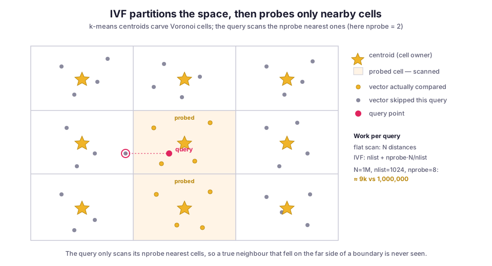
The amount of work saved is the point. Instead of N comparisons, you do nlist to rank the centroids, plus roughly nprobe × N / nlist to scan the probed cells (assuming vectors spread evenly). With a million vectors, nlist = 1024, and nprobe = 8, that is about 1024 + 8,000 comparisons instead of 1,000,000. Two orders of magnitude less work, for an answer that is usually the same.
Building one with FAISS
The FAISS API makes the two-phase shape explicit. You have to train the index (run the k-means) before you can add vectors to it, because there are no cells to add into until the centroids exist. The example builds a cosine-similarity IVF index, adds the corpus, and runs a search:
import faiss
import numpy as np

d = 768            # embedding dimension
nlist = 1024       # number of cells / centroids

quantizer = faiss.IndexFlatIP(d)                 # measures query-to-centroid distance
index = faiss.IndexIVFFlat(quantizer, d, nlist, faiss.METRIC_INNER_PRODUCT)

# train() runs k-means to learn the nlist centroids.
# Use a representative sample, not a corner of the corpus.
train_vectors = load_sample()                    # shape (n_train, 768), n_train >> nlist
faiss.normalize_L2(train_vectors)                # cosine == inner product on unit vectors
index.train(train_vectors)

corpus = load_all_embeddings()                   # shape (N, 768)
faiss.normalize_L2(corpus)
index.add(corpus)                                # assigns each vector to its nearest cell

index.nprobe = 8                                 # search this many cells per query
faiss.normalize_L2(query)
distances, ids = index.search(query, k=10)
Two lines carry most of the meaning. IndexFlatIP as the quantizer means the coarse ranking of centroids is itself an exact flat search, just over nlist centroids instead of N vectors, which is cheap. And index.nprobe = 8 is the one runtime knob that decides the entire speed-versus-accuracy trade. You can change it per query without rebuilding anything, which is the nicest property IVF has.
nprobe is the whole tradeoff
Set nprobe = 1 and you scan only the single closest cell. That is the fastest possible search, and your recall is whatever fraction of the true neighbors happened to live in that one cell. Raise nprobe and you scan more neighboring cells: you catch more of the true neighbors and pay proportionally more time. At nprobe = nlist you scan every cell, which is a flat search with extra steps. It is exact again, and slower than a plain flat index, because you also paid for the partitioning.
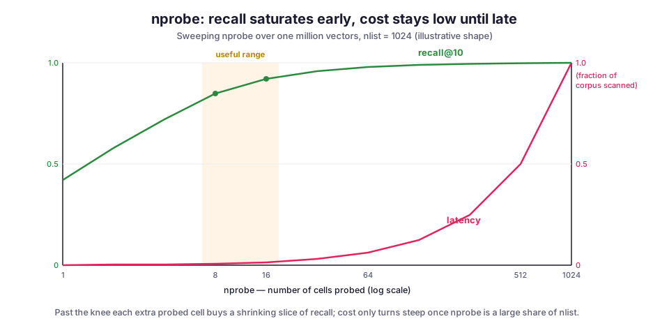
The shape of those two curves is why IVF is worth the trouble. Recall climbs fast and then saturates, while cost keeps rising with every extra cell you probe and never flattens. Between them sits a knee, usually at a small nprobe relative to nlist, where you have bought most of the recall for a fraction of the scanning.
Finding that knee is not guesswork. Build the index, hold out a set of queries, and compute their exact neighbors once with a flat index. Then sweep nprobe while measuring recall@k against that ground truth. The right nprobe is the smallest one that clears your recall target. Nobody can tell you that number from theory; it depends on how your embeddings cluster.
Where it bites
The happy path is a dozen lines. The failure modes all follow from one fact: IVF draws hard boundaries through a continuous space, and hard boundaries cut through neighborhoods.
The boundary problem is structural, not a bug. A query near the edge of its cell has true neighbors sitting just across the line, in a cell you did not probe. That circled, missed point in the first diagram is not a rare accident; it is the built-in cost of partitioning. Raising nprobe shrinks the problem because you probe more of the adjacent cells, which is exactly why recall and nprobe move together. Short of scanning every cell, no nprobe guarantees you caught everything.
The index has to be trained, and training can go wrong. The centroids come from k-means on a sample. Train on an unrepresentative slice, say the first 10,000 vectors when your corpus is sorted by source, and the cells describe that corner of the space instead of the whole thing. Vectors from the rest of the corpus then pile into a handful of ill-fitting cells while others sit nearly empty, and both speed and recall degrade. Sample across the whole corpus, and give k-means enough points: the FAISS guidance suggests on the order of 30 to 256 training points per centroid.
Cells drift as you add data. The centroids are frozen at train time. If your corpus grows or shifts domain after training, new vectors still get assigned to the old cells, and the partition slowly stops matching the data. It is the same staleness the PQ codebooks have. Appending is cheap, but eventually the cells no longer balance, and you have to retrain and re-add. That runs into the incremental indexing tradeoffs: a retrain is a rebuild, not an update.
nlist is a sizing decision, not a default. With too few cells, each posting list is long, so probing a cell scans a lot of vectors and you lose the speedup. With too many, each cell is tiny: the coarse quantizer’s own nlist-way ranking gets expensive, and you need a larger nprobe to gather enough candidates. The common starting point is around sqrt(N) cells, tuned from there. A million vectors lands near nlist = 1024 to 4096.
The metric has to match the embeddings. IVF inherits whatever distance you configure. Text embeddings are almost always compared with cosine, which means normalizing the vectors and using inner product, as in the code above. Get this wrong and both the k-means partition and the search are measuring in the wrong geometry.
IVF-PQ, and how IVF compares with HNSW
IVF narrows how many vectors you compare against. It does nothing about how large each one is, which is why it pairs so naturally with product quantization. IVF picks the candidate cells. PQ stores each vector as a few bytes and scores it with table lookups instead of full dot products. The combination, IVF-PQ, is the workhorse behind large FAISS indexes. It shows up in index factory strings like IVF4096,PQ96, which means: partition into 4096 cells, and encode residuals with 96-byte codes. The original Jégou, Douze, and Schmid paper introduced both pieces together for exactly this reason.
Against HNSW, the tradeoff is fairly settled. HNSW usually gives better recall at a given latency and needs no separate training step, which is why it is the default in a lot of vector databases. IVF wins on memory and build time. The graph’s neighbor lists cost real bytes per vector, while IVF’s overhead is just the posting lists and nlist centroids, and IVF-PQ compresses the vectors on top. IVF is also simpler to shard and to reason about, since a cell is just a list. OpenSearch’s k-NN plugin exposes both through its FAISS engine, so the choice is a config value, not a rewrite. The rough rule:
- Reach for HNSW when recall per millisecond is what you are optimizing and the vectors fit in RAM.
- Reach for IVF-PQ when the corpus is large enough that memory, not query latency, is the binding constraint.
For Archi, the retrieval copilot I worked on for CMS computing operations at CERN, the dense index feeds the vector half of hybrid search. The knowledge base has no natural ceiling, because every logbook entry and ticket is another chunk. IVF is the structure that lets that index answer a query by looking at a few thousand candidates instead of all of them. nprobe is the dial that trades a little recall for a lot of speed once the corpus outgrows a flat scan. The discipline is the same as it was for PQ: keep the flat baseline’s recall next to the approximate index’s, because that gap is the only honest measure of what the partitioning cost you.
Diagrams by M. Hassan Ahmed, released under CC0. No external image was used for this post; the figures are original work by the author.