RAG Vector Search in Postgres with pgvector
Store and query RAG embeddings inside Postgres with pgvector: HNSW indexing, distance operators, metadata filtering, hybrid search, and the tradeoffs I hit.

Most RAG (retrieval-augmented generation) tutorials reach for a dedicated vector database on the first page: Pinecone, Qdrant, Weaviate, Milvus. You pick one, run it next to your app, sync your data into it, and now you have two stores to keep consistent. That’s a reasonable choice at large scale. It’s also a lot of infrastructure to stand up before you’ve proven the retrieval is any good.
If you already run Postgres (and for the backends I build, I almost always do), you can skip that second system entirely. pgvector is a Postgres extension that adds a vector column type and approximate nearest-neighbour indexes. Your embeddings live in the same table as the chunk text and the metadata you filter on. The same pg_dump backs them up, and the same BEGIN/COMMIT makes them transactional. Retrieval becomes one SQL query.
This post is for engineers building a RAG pipeline who want to know whether Postgres is enough before they commit to a separate vector store. It covers the schema, how the distance operators behave, when to use an HNSW index versus IVFFlat, how metadata filtering interacts with the index, and the failure modes that bit me. The examples use FastAPI, because that’s the backend I use in CloudCanvasAI and Archi, the CMS operations copilot I worked on.
Where pgvector sits in a RAG pipeline
RAG has two halves:
- Indexing happens once, ahead of time. Chunking and indexing turn your documents into embeddings.
- Retrieval happens at request time. It embeds the user’s question and finds the chunks whose vectors sit closest to the question’s vector.
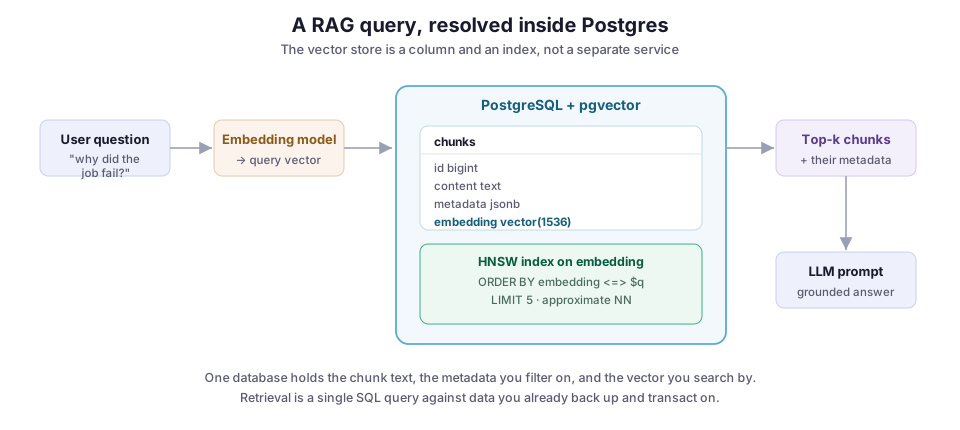
pgvector owns the storage and the retrieval half. The diagram below shows the request path. Nothing in it talks to a vector service: the “vector store” is a column and an index inside the database you already operate.
Setup and schema
Install the extension, then create it once per database:
CREATE EXTENSION IF NOT EXISTS vector;Next, create a table. The dimension in vector(1536) has to match your embedding model exactly. 1536 is the width of OpenAI’s text-embedding-3-small. If you switch models, you re-embed everything, so pin this down before you ingest at scale.
CREATE TABLE chunks (
    id         BIGINT GENERATED ALWAYS AS IDENTITY PRIMARY KEY,
    document   TEXT        NOT NULL,   -- source doc id, for citations
    content    TEXT        NOT NULL,   -- the chunk itself
    metadata   JSONB       NOT NULL DEFAULT '{}',
    embedding  VECTOR(1536)
);
Keeping content and metadata in the same row as embedding is the whole point. When a query returns, you already have the text to feed the model and the source id to cite. There is no second lookup keyed on an external vector-store id that you have to keep in sync.
Writing embeddings from FastAPI
pgvector’s Python bindings register the vector type with your database driver, so you can pass a plain Python list. With asyncpg and the pgvector package, an insert helper looks like this:
import asyncpg
from pgvector.asyncpg import register_vector

async def store_chunks(pool, doc_id: str, chunks: list[str], vectors: list[list[float]]):
    async with pool.acquire() as conn:
        await register_vector(conn)
        await conn.executemany(
            "INSERT INTO chunks (document, content, embedding) VALUES ($1, $2, $3)",
            [(doc_id, text, vec) for text, vec in zip(chunks, vectors)],
        )
Batch the inserts. The embedding API calls dominate ingest latency, not the database writes. So the pattern that matters is: embed a batch of chunks in one API call, then executemany them in one round trip.
Querying with the distance operators
Retrieval is an ORDER BY ... LIMIT k. pgvector exposes distance as operators, and the operator you pick has to match how your embeddings were trained:
<=>cosine distance<->L2 (Euclidean) distance<#>negative inner product<+>L1 (taxicab) distance
Most embedding models, including OpenAI’s and the common open-weight ones, produce vectors normalized to unit length and are meant to be compared by cosine similarity. So <=> is the usual answer.
One detail trips people up: pgvector returns cosine distance, which is 1 - cosine_similarity. Smaller means closer, so you sort ascending. If you want a similarity score to threshold on, compute 1 - (embedding <=> $1) yourself, as the search function below does:
async def search(pool, query_vec: list[float], k: int = 5):
    async with pool.acquire() as conn:
        await register_vector(conn)
        rows = await conn.fetch(
            """
            SELECT document, content,
                   1 - (embedding <=> $1) AS similarity
            FROM chunks
            ORDER BY embedding <=> $1
            LIMIT $2
            """,
            query_vec, k,
        )
        return [dict(r) for r in rows]
You pass the query vector once and reference it as $1 in both the SELECT and the ORDER BY. The planner is smart enough not to compute the distance twice.
Indexing: without one, every query is a full scan
The query above works on day one. By the time you have a few hundred thousand rows, it has quietly become your bottleneck. With no index, Postgres computes the distance to every row on every query. That is an exact, linear scan: correct, and slow.
pgvector offers two approximate indexes. Both skip most of the rows, trading a small amount of recall (the share of true nearest neighbours you get back) for a large speedup.
HNSW, the default
HNSW (Hierarchical Navigable Small World) builds a multi-layer graph that the search navigates greedily toward the nearest neighbours. It’s the one I default to: it gives better recall at a given speed, and it doesn’t need training data to exist first. The costs are a slower build and more memory. This is the same HNSW algorithm I broke down in an earlier post, now as a Postgres index.
CREATE INDEX ON chunks
USING hnsw (embedding vector_cosine_ops)
WITH (m = 16, ef_construction = 64);
Two things to get right in that statement:
- The operator class must match your query operator.
vector_cosine_opsgoes with<=>,vector_l2_opswith<->, andvector_ip_opswith<#>. Mismatch them and the planner quietly ignores the index and falls back to a full scan. - The build parameters.
m(16 by default) is the number of connections per node.ef_construction(64 by default) is how hard the builder searches while inserting. Higher values mean better recall and a slower, heavier build.
IVFFlat, and its sharp edge
IVFFlat partitions vectors into lists clusters and searches only the nearest few. It builds faster and uses less memory, but its recall is more sensitive to tuning.
Here is the sharp edge: IVFFlat learns its clusters from the rows present at build time. So you have to build it after you have a representative sample of data. Load data first, then index.
Tuning recall at query time
At query time, HNSW has a knob that controls the recall/latency tradeoff for the session:
SET hnsw.ef_search = 100; -- default is 40; higher = better recall, slowerRaise it when you’re missing relevant chunks. Lower it when p99 latency matters more than the last few points of recall. Measure this against a labelled set rather than eyeballing it. I wrote about how to measure retrieval quality precisely because “it feels better” is not a number you can regress against.
Metadata filtering, and the trap inside it
Real retrieval is rarely “search all chunks.” You want this user’s documents, or only pages from the current release, or entries after some date. That’s a WHERE clause on the jsonb column:
SELECT document, content
FROM chunks
WHERE metadata->>'project' = 'wmcore'
ORDER BY embedding <=> $1
LIMIT 5;
Here’s the part that surprises people: the HNSW index knows nothing about your WHERE clause. Postgres walks the vector index in nearest-first order and then discards rows that fail the filter.
Suppose your filter is selective and keeps only 2% of rows. The index can hand back its whole candidate list before it finds five rows that pass. You then quietly get fewer than five results, or a slow query as the scan reaches deeper.
pgvector’s answer is iterative index scans (added in 0.8.0). They let the scan go back and pull more candidates when the filter is strict:
SET hnsw.iterative_scan = strict_order;Even so, if you always filter on the same high-cardinality field, partial indexes or partitioning by that field will beat a single global index. Push the selective, structured constraint into something Postgres can index conventionally, and let the vector index do the semantic part on the smaller set.
Dedicated vector databases wrap this same tradeoff in a “metadata filter” feature. In Postgres you see the mechanism directly, which is either a burden or a gift depending on your mood that day.
Hybrid search comes almost for free
Vector search misses exact matches. Ask for error code HTTP 431 or a specific dataset name, and semantic similarity will happily return chunks that are about errors without containing the token you need.
Postgres already ships full-text search. So you can run keyword and vector retrieval in the same database and fuse the rankings, with no second service or query engine. The keyword half is a standard full-text query:
SELECT id, content
FROM chunks
WHERE to_tsvector('english', content) @@ plainto_tsquery('english', $1)
LIMIT 20;
Combining that lexical result with the vector result, usually with Reciprocal Rank Fusion, is the hybrid search pattern I covered in its own post. The point here is that pgvector doesn’t force you to choose: both retrievers read the same table.
Failure modes I’ve actually hit
- The index that isn’t used. The operator class doesn’t match the query operator, or you wrapped the column in a function, and the planner drops to a sequential scan. Run
EXPLAIN ANALYZEand look forIndex Scan using ..._hnsw. If you seeSeq Scan, the index is decorative. - Dimension drift. You changed embedding models, and the new vectors are 3072-dim against a
vector(1536)column. The insert errors. The subtler version is comparing vectors from two different models: the spaces don’t align, so you get confidently wrong neighbours. - Distance sign confusion.
<#>returns the negative inner product so that “smaller is closer” holds for the index. If you treat it as a raw similarity, you’ll rank everything backwards. - Memory during build. HNSW builds hold the graph in
maintenance_work_mem. On a large table with the default setting, the build spills and crawls. Raisemaintenance_work_memfor the session beforeCREATE INDEX, then set it back. - Recall you never measured. Approximate indexes are approximate, and the full scan is your ground truth. Sample a few hundred queries, compare the index results against the exact ones, and know your recall number before you tune
ef_searchin the dark.
What I’d do differently, and where the line is
For a first RAG system, I’d start in Postgres every time. I’d move to a dedicated vector store only when a concrete number forces it:
- index builds that take longer than your ingest window;
- memory that won’t fit the box;
- query volume that needs horizontal sharding a single Postgres node can’t give you.
Those are real limits, and pgvector doesn’t pretend otherwise. But most projects reach “good enough retrieval” long before they hit those walls. Every week spent operating a second datastore is a week not spent improving chunking, reranking, and evaluation, which is where retrieval quality actually comes from.
The one thing I’d do earlier than I used to: raise maintenance_work_mem, and set hnsw.ef_search deliberately from a measured recall target, not by feel. Both are one line, and together they are the difference between “the demo works” and “retrieval holds up under a real query load.”
For the projects behind this post (the retrieval layer in Archi and the document backends in CloudCanvasAI), keeping vectors in Postgres has meant one system to reason about, back up, and transact against. The best infrastructure decision is often the one that leaves you fewer moving parts to break.
References
- pgvector: the extension, README, and changelog
- pgvector-python: bindings for psycopg, asyncpg, SQLAlchemy, and more
- PostgreSQL full-text search: the lexical half of hybrid retrieval
- Malkov & Yashunin, Efficient and robust approximate nearest neighbor search using HNSW graphs: the algorithm behind the index