HyperLogLog: Count Distinct at Scale in 12KB
Counting unique items exactly costs memory that grows with your data. HyperLogLog estimates the cardinality of billions in about 12KB. Here's how it works.

How many distinct things are in this stream? Distinct users today, distinct error signatures this hour, distinct workflow IDs that touched a broken storage endpoint. The question sounds trivial until you try to answer it fast. The exact answer requires remembering everything you have already seen, so that you never count it twice, and “remember everything” is the part that does not scale.
I hit this on the telemetry side of CMS workflow operations at CERN. The logs from WMCore and its surrounding databases are large enough that a plain COUNT(DISTINCT) over a wide time range either times out or quietly eats a node’s heap. HyperLogLog is the algorithm that sidesteps this. It answers “how many unique?” for billions of items using a fixed slab of memory measured in kilobytes, and its summaries can be combined across shards. The catch is that the answer is an estimate.
This post is for engineers who need distinct counts at a scale where exact counting is no longer an option, and who want to know what they are trading away. It covers why exact counting breaks, how HyperLogLog works, why it merges so well, how to use it in Redis and OpenSearch, and where it misleads you.
Why exact counting stops scaling
The obvious way to count uniques is a set. Walk the stream, drop every item into a hash set, and the size of the set is your answer. It is exact and simple. Its memory cost is the problem: the set must hold one entry per unique value, so it grows with the number of distinct items.
Ten million unique 20-byte workflow IDs already make a couple hundred megabytes of set, before overhead. Do that for fifty different metrics across a retention window, and you are budgeting real RAM for a question nobody needs a byte-perfect answer to.
Distribution makes it worse. When your data lives on many shards, each shard can build its own set. But to get the global distinct count you have to merge those sets, which means shipping every ID to one place and de-duplicating there. You have moved the whole dataset across the network just to count it.
That is the wall. What you want instead is a small, fixed-size summary of a set that you can merge cheaply. That is exactly what a HyperLogLog sketch is. (A sketch is a compact data structure that summarizes a large dataset and answers approximate queries about it.)
The core idea: rare bit patterns hint at large counts
The whole family of algorithms rests on a bet about randomness. Run each item through a good hash function, so its output looks like uniform random bits. Then look at how many zero bits the hash starts with:
- About half of random hashes start with a
1, so no leading zeros. - A quarter start with
01. - An eighth start with
001.
A hash that begins with ten leading zeros is a one-in-a-thousand event. If you have seen one, you have probably looked at something on the order of a thousand distinct values.
That is the entire intuition, and it goes back to Flajolet and Martin’s 1985 probabilistic counting work. Track the maximum number of leading zeros you have seen across all items, call it ρ, and 2^ρ is a rough guess at the cardinality (the number of distinct items).
“Rough” is the key word. A single unlucky hash with a long run of zeros throws the estimate off by a factor of two, because the whole count rests on one extreme observation. HyperLogLog’s real contribution is not the leading-zeros idea. It is how it beats down that variance while storing only a few kilobytes.
Many registers, combined with a harmonic mean
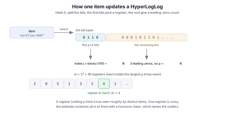
Instead of one running maximum, HyperLogLog keeps many. It splits each hash into two parts:
- The first p bits select one of
m = 2^pregisters (small counters). - The remaining bits are where it counts leading zeros.
Each register stores the largest leading-zero count (plus one) that any item routed to it has produced. You are now running m independent little experiments in parallel, and each register is one noisy estimator. The diagram walks through a single update.
Combining the registers
The way HyperLogLog combines the registers is where it earns its name. You might expect an ordinary average, but an arithmetic mean is still wrecked by the occasional huge register. Instead, HyperLogLog takes the harmonic mean of 2 raised to each register value, scaled by a correction constant. The harmonic mean is dominated by the small values, so it shrugs off large outliers. The published estimator is:
E = α_m · m² / Σ_j 2^(−M[j])Here M[j] is the value in register j, and α_m is a constant near 0.7213 that corrects the systematic bias of the raw formula. You do not need to memorize the formula.
The one tuning knob: error versus memory
The property that matters falls out of the formula: with m registers, the standard error is about 1.04 / √m. Quadruple the registers and you halve the error. That relationship is the entire tuning knob, and it explains the numbers you see in real systems. Here is how it plays out in Redis:
- Redis uses
m = 16384registers. 1.04 / √16384 = 1.04 / 128, which is0.0081: the 0.81% error its docs quote.- Each register only needs to hold a number up to about 64, so six bits is plenty.
16384 × 6 bitsis12288bytes: the famous 12KB.
That memory is fixed whether you feed the sketch a thousand items or a trillion.
The add path
Written out, adding an item is unremarkable, which is the point. Hash the item, use the top bits to pick a register, count leading zeros in the rest, and keep the maximum:
def add(self, item):
    h = hash64(item)                    # a good 64-bit hash
    j = h >> (64 - self.p)              # first p bits -> register index
    w = (h << self.p) & MASK_64        # the rest of the bits
    rho = leading_zeros(w) + 1         # position of the leftmost 1
    self.registers[j] = max(self.registers[j], rho)
Every add is constant time and touches one register. There is no growth, no rehashing, no compaction.
Why sketches merge, and why that is the real win
The register update is a max, and that one detail is what makes HyperLogLog usable in a distributed system. You can merge two sketches built over two different slices of data by taking the larger of the two values at each register position. The result is bit-for-bit the sketch you would have gotten by feeding both slices into one HyperLogLog from the start.
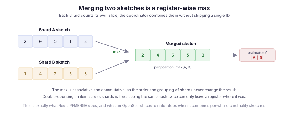
Two properties of max make this safe:
- Order does not matter.
maxis associative and commutative, so neither the order you merge shards in nor how you group them can change the answer. - Duplicates are harmless. An item that shows up on two shards is not double-counted. Its hash produces the same
ρin the same register on both, andmax(ρ, ρ)isρ.
This is why a query engine can have each shard compute a tiny local sketch, ship only the sketch to a coordinator, and combine them there. You send twelve kilobytes per shard instead of the whole dataset. Redis exposes this directly as PFMERGE. OpenSearch does it internally every time you run a distributed cardinality aggregation.
Using it in Redis and OpenSearch
You rarely implement HyperLogLog yourself, because the systems you already run ship it.
Redis
In Redis, HyperLogLog is three commands, available since 2.8.9. The example adds three IDs (one repeated) to a daily key, reads the count, and rolls two days into a weekly key:
PFADD workflows:2026-09-26 wf-4487 wf-4488 wf-4487
PFCOUNT workflows:2026-09-26          # -> 2, wf-4487 counted once
PFMERGE workflows:week workflows:2026-09-26 workflows:2026-09-25PFADDfolds items into the sketch.PFCOUNTreads the estimate.PFMERGEunions sketches into a new key. That is how you roll daily counts up into a weekly one without ever storing the IDs.
OpenSearch
In OpenSearch, the same machinery sits behind the cardinality aggregation. It uses HyperLogLog++, Google’s refinement of the original with 64-bit hashes and a sparse layout for small counts. This query counts distinct workflow IDs across the log indexes:
GET logs-*/_search
{
  "size": 0,
  "aggs": {
    "distinct_workflows": {
      "cardinality": {
        "field": "workflow_id",
        "precision_threshold": 3000
      }
    }
  }
}
The precision_threshold is the same error-versus-memory knob from earlier, under a different name. Counts at or below the threshold are near-exact. Above it, you get the HyperLogLog estimate, which OpenSearch documents as typically within about 6% of the true value. The default is 3000 and the maximum is 40000. Raising it buys accuracy with memory, in the same 1.04/√m trade.
For a dashboard panel showing “distinct failing workflows over the last 24 hours,” the default is usually fine. Being off by a few percent on a trending number is not the kind of error that misleads anyone.
Where it bites
The estimate is the honest tradeoff, but a few sharper edges catch people.
The error is relative, not absolute. A 1% standard error on a true count of 50 million is a swing of half a million. That is fine for a trend line and wrong for anything you would put in a billing row or a compliance report. Distinct counts that feed money or audits need exact counting, full stop.
A sketch cannot list its members. It counts; it does not enumerate. If the next question after “how many distinct workflows failed?” is “which ones?”, a HyperLogLog has nothing to give you, because it never stored them. Use it for the count, and go back to the source when you need the list.
Intersections are a trap. Union is exact and cheap, but there is no direct way to intersect two sketches. The usual workaround is inclusion-exclusion, |A ∩ B| = |A| + |B| − |A ∪ B|. It combines the errors of three separate estimates, so it degrades badly when the sets are similar in size and the overlap is small. If you genuinely need set intersections at scale, HyperLogLog is the wrong tool; something like a MinHash sketch fits better.
Small cardinalities were the original weak spot. The raw estimator is biased low when the true count is small relative to the number of registers. That is precisely why HyperLogLog++ added empirical bias correction and a sparse representation for that range. Redis and OpenSearch already include those fixes. If you hand-roll from the 2007 paper, you will see the low-end skew yourself.
Everything rests on the hash. HyperLogLog assumes the hash spreads inputs uniformly across the bit space. A weak hash, or one with structure in the high bits you use to pick registers, breaks that assumption, and the estimate drifts. Use a hash designed for even distribution: not a cryptographic one you picked for other reasons, and not something homegrown.
What I use it for
HyperLogLog earns its keep on the dashboard question that would otherwise be a full scan: distinct workflows, distinct users, or distinct error fingerprints over a time range wide enough that exact counting is off the table. It fits naturally into an observability setup. I have written about building OpenSearch dashboards to watch workflow health and about keeping the indexes behind them from filling a disk. Cardinality panels are the natural next thing to put on those dashboards. Now you know the sketch doing the counting and, more usefully, when to stop trusting it.
The pattern generalizes past this one algorithm. A fixed-size, mergeable summary that answers a question approximately is often worth far more than an exact answer you cannot afford to compute. Distinct counts are just the cleanest example.
Diagrams by M. Hassan Ahmed, released under CC0. No external image was used for this post; the figures are original work by the author.