How Speculative Decoding Speeds Up LLM Inference
Speculative decoding uses a small draft model to guess tokens a big model verifies in one pass, cutting LLM latency 2-3x without changing the output.

Watch a large language model generate text on a GPU and something looks wrong. The card is expensive and the model is loaded, yet utilization sits low while tokens trickle out one at a time. The GPU is not the bottleneck. The problem is that autoregressive decoding is serial: to produce token N, the model needs token N-1. So you run one full forward pass per token, no matter how much compute sits idle.
I ran into this building the answer path for Archi, the RAG (retrieval-augmented generation) copilot I worked on for CMS computing operations at CERN. Retrieval was fast and the model was fine, but a long answer still felt slow, because every token was another trip through a 7-billion-parameter network.
This post is for engineers who serve LLMs and want lower latency without switching to a smaller, dumber model. Speculative decoding buys exactly that. It works because of a nice piece of systems thinking: it turns a memory-bandwidth problem into a compute problem, on hardware that has compute to spare. The sections below cover why single-token decoding wastes the GPU, how the draft-and-verify loop works, why it doesn’t change the output, what sets the speedup, and where it breaks.
Why single-token decoding wastes the card
The earlier post on the KV cache covered where GPU memory goes during generation. The other half of the story is bandwidth. During decode, each step reads the entire model’s weights out of high-bandwidth memory to produce exactly one token. For a 7B model in fp16 (16-bit floats, two bytes per weight), that is roughly 14 GB moved per token. The arithmetic the GPU does with those weights is tiny by comparison, so the step finishes long before the compute units are busy. Decode is memory-bandwidth bound: you pay to shuttle weights, not to do math.
That framing points straight at the fix. If reading the weights is the cost and the math is nearly free, then checking many candidate tokens in one weight read costs almost the same as checking one. A single forward pass over K positions produces a next-token distribution at every one of those positions in parallel, in about the same wall-clock time as a single-token step.
Autoregressive decode throws that parallelism away, because it doesn’t know tokens 2 through K yet. Speculative decoding gets them from somewhere cheap, then spends that one nearly free parallel pass verifying them.
Draft, then verify
The idea was introduced by Leviathan et al. at ICML 2023 and, independently, by Chen et al. at DeepMind. It uses two models:
- A small, fast draft model guesses the next few tokens, cheaply and one at a time.
- The large target model, the one whose output you actually want, checks all of those guesses in a single forward pass.
Each step runs like this:
- The draft proposes K tokens.
- The target scores them in parallel and accepts the longest prefix it agrees with, stopping at the first token it would not have produced.
- The target replaces that rejected token with one it samples itself, so every step ends with a corrected sequence.
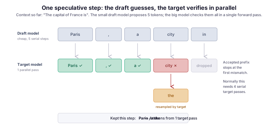
The payoff is fewer expensive target passes. If the draft is right most of the time, you produce several tokens per target pass instead of one, and the target pass is the part you were paying for.
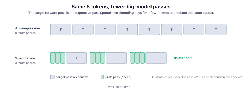
The surprising part: the output doesn’t change
The natural worry is that a small draft model drags down quality. It doesn’t, and that is what makes the technique worth using rather than a quality-for-speed trade.
The acceptance test is a modified form of rejection sampling that provably preserves the target model’s output distribution. It works token by token:
- Accept each drafted token with probability
min(1, p_target / p_draft), where eachpis the probability that model gave the token. - If a token is rejected, resample from the normalized difference between the two distributions, and stop there.
The math guarantees that the tokens you keep are distributed exactly as if the target model had generated them alone. Under greedy decoding (always taking the most likely token), the output is token-for-token identical. Under sampling, it matches the target’s distribution.
So the draft model affects only speed, never what comes out. A better draft gets more tokens accepted per step. A worse one just falls back toward one token at a time. You never trade correctness for it.
Here is the loop with the accounting made explicit. The numbered comments follow the steps above: draft, score everything in one pass, walk the proposals, and collect a bonus token if nothing was rejected.
def speculative_step(context, draft, target, K):
    # 1. Draft proposes K tokens, cheaply and serially.
    proposals, p_draft = draft.generate(context, k=K)

    # 2. Target scores all K positions in ONE forward pass.
    #    p_target[i] is the target's distribution at position i.
    p_target = target.forward(context + proposals)

    # 3. Walk the proposals, accepting the agreed prefix.
    accepted = []
    for i, tok in enumerate(proposals):
        ratio = p_target[i][tok] / p_draft[i][tok]
        if random() < min(1.0, ratio):
            accepted.append(tok)          # target agrees, keep it
        else:
            # First disagreement: resample from the corrected
            # distribution and stop. This is what keeps the
            # output faithful to the target model.
            fixed = normalize(relu(p_target[i] - p_draft[i]))
            accepted.append(sample(fixed))
            return accepted
    # 4. All K accepted: the target's pass also gave us a free
    #    bonus token at position K+1.
    accepted.append(sample(p_target[K]))
    return accepted
Two details are easy to miss:
- The bonus token in step 4 is real. When the target accepts the whole draft, its single pass has already computed a distribution one position past the draft. You get that token for free, so a full step yields up to
K + 1tokens. - A rejection isn’t wasted work either. The resampled correction is still a valid target token. The worst case is one accepted token per step, which is exactly plain autoregressive decoding plus the draft’s overhead.
What determines the speedup
Two numbers set how much you gain, and they pull against each other.
Acceptance rate is the fraction of drafted tokens the target keeps. It reflects how well the draft model imitates the target on your traffic. A draft from the same family (say a 1B model drafting for a 7B one) gets far more accepted than an unrelated small model. Predictable text, such as boilerplate or code with obvious continuations, pushes acceptance up. High-entropy, genuinely creative generation pushes it down.
Draft cost is the price of guessing. Every draft token is a small forward pass, and it is pure overhead whenever the target rejects it. Guess too many tokens per step and, on hard passages, you burn draft compute that gets thrown away. Guess too few and you leave speedup on the table when the draft is doing well.
The reported numbers land in a consistent range. Leviathan et al. measured 2-3x on their setups, and DeepMind reported 2 to 2.5x on Chinchilla 70B with no change in sample quality. That is the honest expectation: a meaningful cut in latency, not an order of magnitude, and it depends on your model pair and your workload.
Variants that don’t need a second model
A separate draft model is the classic formulation, and its annoyance is real. You have to find or train a small model that matches your target, load it, and keep it in memory. Several later methods drop that requirement:
- Medusa (Cai et al.) adds extra decoding heads to the target model itself, each predicting one position further ahead, and verifies the candidates as a tree. No second model, one set of weights.
- N-gram / prompt lookahead skips the model entirely for drafting. It proposes continuations by matching against text already in the prompt or recent output. It costs almost nothing and works surprisingly well when the answer quotes the input, which is common in RAG and summarization.
- Self-speculative approaches draft with a subset of the target’s own layers, again avoiding a separate model.
You rarely implement any of this yourself. vLLM supports draft-model, n-gram, and Medusa-style speculation behind a config flag, and Hugging Face Transformers ships the same idea as assisted generation. The engineering that is actually yours: choosing the draft, setting K, and measuring whether it helps on your traffic.
Where it breaks
High batch sizes erode the win. This is the one that catches people. Speculative decoding spends extra compute to cut serial steps, which pays off when you’re memory-bandwidth bound: the low-batch, single-stream case. As you batch more requests together, the GPU shifts toward compute-bound, the spare compute that made verification “free” is no longer spare, and the extra draft-and-verify FLOPs (floating-point operations) start costing real time. A server already saturating its GPU with a large batch may see little or negative benefit. Speculative decoding is a latency tool for the under-loaded regime, not a throughput tool for the saturated one.
A mismatched draft is worse than none. If acceptance is low, you pay the draft’s overhead on every rejected token and gain almost nothing. The draft has to genuinely track the target on your data, and the only way to know is to measure acceptance on real prompts, not a demo.
Sampling temperature moves acceptance. Higher temperature flattens the target distribution, so the draft and target disagree more often and acceptance drops. The technique shines brightest at low temperature and with greedy decoding. Conveniently, those are exactly the settings a factual RAG assistant tends to run at.
Memory isn’t free. A separate draft model puts more weights on the card, competing with the KV cache for the space the KV cache post was all about. Medusa and self-speculative variants sidestep this, which is a real reason to prefer them.
Tradeoffs, and what I would reach for
If you serve a single-stream or low-concurrency workload where latency matters, speculative decoding is close to free quality-wise and worth turning on. Here is how I’d choose a variant:
- Start with n-gram or prompt lookahead. It needs no second model. For anything that echoes its input (which RAG answers constantly do when they quote a retrieved chunk), it lands a lot of accepted tokens for nearly zero cost.
- Reach for a real draft model when you need more and can pair one from the same family.
- Reach for Medusa when you’d rather not manage a second model at all.
If instead you’re throughput-bound and already keeping the GPU busy with large batches, spend your effort on batching and memory before speculation, because speculation gives that regime the least. Whichever variant you pick, measure the acceptance rate on your own prompts. It is the single number that decides whether any of this is worth it, and it is workload-specific enough that no blog post, including this one, can tell you what yours will be.
For the CERN tooling, the pieces that benefit are the interactive ones. A shift operator waiting on an Archi answer and the code context that LLM DevMate feeds a model are both single requests, where latency is what the person feels. The batch analytics behind the workflow operations console care about throughput instead, and there the ordering is reversed. Same technique, opposite priority: knowing which regime you’re in is most of the decision.
Diagrams by M. Hassan Ahmed, released under CC0. No external image was used for this post; the figures are original work by the author.